In [1]:

import pandas as pd, seaborn as sns, numpy as np
sns.set(font='Bitstream Vera Sans')
sns.set_context('poster', {'figsize':(12,8)})

pd.options.display.max_rows = 8

%matplotlib inline

%cd ~/2014_fall_ASTR599/notebooks/
%run talktools.py
%cd ~/notebook/

[Errno 2] No such file or directory: '/Users/jakevdp/2014_fall_ASTR599/notebooks/'
/Users/jakevdp/Opensource/2014_fall_ASTR599/notebooks

[Errno 2] No such file or directory: '/Users/jakevdp/notebook/'
/Users/jakevdp/Opensource/2014_fall_ASTR599/notebooks

This notebook was put together by Abraham Flaxman for UW's Astro 599 course. Source and license info is on GitHub.

In [2]:

import pandas as pd

big data?¶

medium data¶

learning objectives:¶

know that pandas exists --- tool for manipulating medium sized tabular data
know how to learn more about pandas
get some hands on experience with the pandas.DataFrame for data manipulation

pandas exists¶

(from https://www.openhub.net/p/py-pandas)

In [3]:

import pandas as pd  # we did this already!
# did it work?

In [4]:

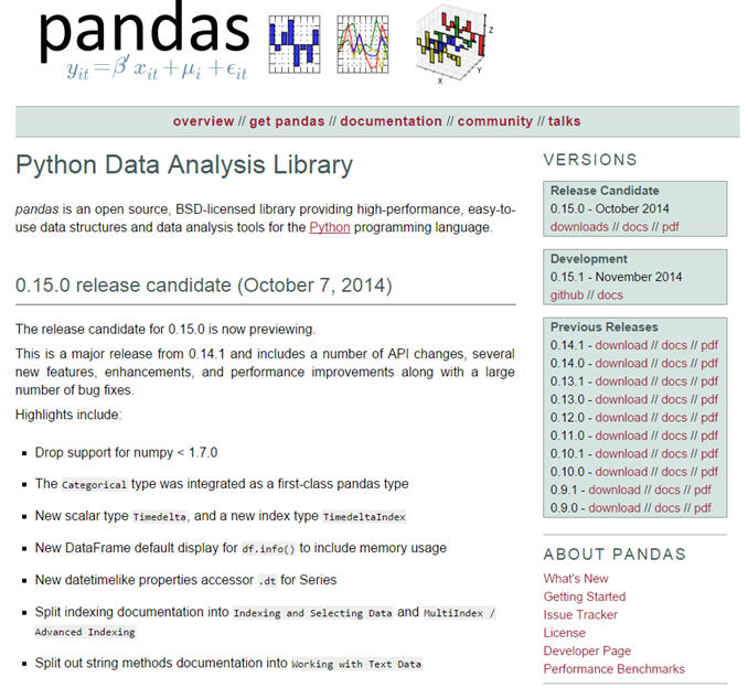
pd.__version__

Out[4]:

'0.14.1'

how to learn more¶

In [ ]:

pd.DataFrame([shift-tab]

hands on experience¶

making DataFrames
using tabular data
reshaping tables
combining tables
grouping, mapping, and applying
dealing with date and time data

making `DataFrames`¶

In [6]:

# loading a csv
df = pd.read_csv(fname)

---------------------------------------------------------------------------
NameError                                 Traceback (most recent call last)
<ipython-input-6-30775157dcae> in <module>()
      1 # loading a csv
----> 2 df = pd.read_csv(fname)

NameError: name 'fname' is not defined

In [ ]:

# loading an excel file
df = pd.read_[tab]

In [ ]:

# loading a stata file
df = pd.read_

making `DataFrames` from scratch¶

In [7]:

df = pd.DataFrame({'a': [10,20,30],
                   'b': [40,50,60]})

In [8]:

df

Out[8]:

	a	b
0	10	40
1	20	50
2	30	60

In [18]:

# think of DataFrames as numpy arrays plus
df.columns
df.index
df.b.index is df.index

Out[18]:

True

questions?¶

aside: global health¶

our running example¶

From Global Health Data Exchange, load PHMRC VA adult data, CSV format:

In [19]:

url = 'http://ghdx.healthdata.org/sites/default/files/'\
      'record-attached-files/IHME_PHMRC_VA_DATA_ADULT_Y2013M09D11_0.csv'

In [20]:

df = pd.read_csv(url)

/Users/jakevdp/anaconda/lib/python2.7/site-packages/pandas/io/parsers.py:1139: DtypeWarning: Columns (18,29,38,41,60,96) have mixed types. Specify dtype option on import or set low_memory=False.
  data = self._reader.read(nrows)

In [21]:

df = pd.read_csv(url, low_memory=False)

what's in `df`?¶

In [22]:

df

Out[22]:

	site	module	gs_code34	gs_text34	va34	gs_code46	gs_text46	va46	gs_code55	gs_text55	...	word_woman	word_womb	word_worri	word_wors	word_worsen	word_worst	word_wound	word_xray	word_yellow	newid
0	Mexico	Adult	K71	Cirrhosis	6	K71	Cirrhosis	8	K71	Cirrhosis	...	0	0	0	0	0	0	0	0	0	1
1	AP	Adult	G40	Epilepsy	12	G40	Epilepsy	16	G40	Epilepsy	...	0	0	0	0	0	0	0	0	0	2
2	AP	Adult	J12	Pneumonia	26	J12	Pneumonia	37	J12	Pneumonia	...	0	0	0	0	0	0	0	0	0	3
3	Mexico	Adult	J33	COPD	8	J33	COPD	10	J33	COPD	...	0	0	0	0	0	0	0	0	0	4
...	...	...	...	...	...	...	...	...	...	...	...	...	...	...	...	...	...	...	...	...	...
7837	Dar	Adult	ZZ23	Other Cardiovascular Diseases	22	ZZ23	Other Cardiovascular Diseases	31	ZZ23	Other Cardiovascular Diseases	...	0	0	0	0	0	0	0	0	0	7843
7838	AP	Adult	T36	Poisonings	27	T36	Poisonings	38	T36	Poisonings	...	0	0	0	0	0	0	0	0	0	7844
7839	UP	Adult	X09	Fires	15	X09	Fires	19	X09	Fires	...	0	0	0	0	0	0	0	0	0	7845
7840	Dar	Adult	C15	Esophageal Cancer	13	C15	Esophageal Cancer	17	C15	Esophageal Cancer	...	0	0	0	0	0	0	0	0	0	7846

7841 rows × 946 columns

In [23]:

# also load codebook (excel doc)
url = 'http://ghdx.healthdata.org/sites/default/files/'\
      'record-attached-files/IHME_PHMRC_VA_DATA_CODEBOOK_Y2013M09D11_0.xlsx'
cb = pd.read_excel(url)

In [27]:

cb.head()

Out[27]:

	variable	question	module	coding
0	site	Site	General	NaN
1	newid	Study ID	General	NaN
2	gs_diagnosis	Gold Standard Diagnosis Code	General	NaN
3	gs_comorbid1	Gold Standard Comorbid Conditions 1	General	NaN
4	gs_comorbid2	Gold Standard Comorbid Conditions 2	General	NaN

using tabular data¶

In [29]:

# each column of pd.DataFrame is a pd.Series
cb.module

Out[29]:

0    General
1    General
...
1647    Neonate
1648    Neonate
Name: module, Length: 1649, dtype: object

In [44]:

# can uses square-brackets instead of "dot"
# (useful if column name has spaces!)
cb.iloc[3, 3]

Out[44]:

In [45]:

# what's in this series?
cb.module.value_counts()

Out[45]:

Adult      902
Child      466
Neonate    218
General     63
dtype: int64

In [46]:

# accessing individual cells
df.head()

Out[46]:

	site	module	gs_code34	gs_text34	va34	gs_code46	gs_text46	va46	gs_code55	gs_text55	...	newid
0	Mexico	Adult	K71	Cirrhosis	6	K71	Cirrhosis	8	K71	Cirrhosis	...	1
1	AP	Adult	G40	Epilepsy	12	G40	Epilepsy	16	G40	Epilepsy	...	2
2	AP	Adult	J12	Pneumonia	26	J12	Pneumonia	37	J12	Pneumonia	...	3
3	Mexico	Adult	J33	COPD	8	J33	COPD	10	J33	COPD	...	4
4	UP	Adult	I21	Acute Myocardial Infarction	17	I21	Acute Myocardial Infarction	23	I21	Acute Myocardial Infarction	...	5

5 rows × 946 columns

In [47]:

# to access by row and column
# can use names
df.loc[4, 'gs_text34']

Out[47]:

'Acute Myocardial Infarction'

In [48]:

# or use numbers
df.iloc[4, 3]

Out[48]:

'Acute Myocardial Infarction'

In [49]:

# same because columns 3 is gs_text
# how to check?
df.columns[3]

Out[49]:

'gs_text34'

improve this example¶

In [50]:

df.head()

Out[50]:

	site	module	gs_code34	gs_text34	va34	gs_code46	gs_text46	va46	gs_code55	gs_text55	...	newid
0	Mexico	Adult	K71	Cirrhosis	6	K71	Cirrhosis	8	K71	Cirrhosis	...	1
1	AP	Adult	G40	Epilepsy	12	G40	Epilepsy	16	G40	Epilepsy	...	2
2	AP	Adult	J12	Pneumonia	26	J12	Pneumonia	37	J12	Pneumonia	...	3
3	Mexico	Adult	J33	COPD	8	J33	COPD	10	J33	COPD	...	4
4	UP	Adult	I21	Acute Myocardial Infarction	17	I21	Acute Myocardial Infarction	23	I21	Acute Myocardial Infarction	...	5

5 rows × 946 columns

In [51]:

# make the row names more interesting than numbers starting from zero
df.index = ['person %d'%(i+1) for i in df.index]

In [52]:

# have a look at the first ten rows and first five columns
df.iloc[:10, :5]

Out[52]:

	site	module	gs_code34	gs_text34	va34
person 1	Mexico	Adult	K71	Cirrhosis	6
person 2	AP	Adult	G40	Epilepsy	12
person 3	AP	Adult	J12	Pneumonia	26
person 4	Mexico	Adult	J33	COPD	8
...	...	...	...	...	...
person 7	Dar	Adult	N17	Renal Failure	29
person 8	Dar	Adult	B20	AIDS	1
person 9	Bohol	Adult	C34	Lung Cancer	19
person 10	UP	Adult	O67	Maternal	21

10 rows × 5 columns

In [53]:

# slicing with named indices is possible, too
df.loc['person 10', 'site':'gs_text34']

Out[53]:

site               UP
module          Adult
gs_code34         O67
gs_text34    Maternal
Name: person 10, dtype: object

notice anything weird about that, though?

what else can we do?¶

In [54]:

# logical operations (element-wise)
df.module == "Adult"

Out[54]:

person 1    True
person 2    True
...
person 7840    True
person 7841    True
Name: module, Length: 7841, dtype: bool

In [55]:

# usefule for selecting subset of rows
dfa = df[df.module == "Adult"]

In [56]:

# summarize
dfa.va34.describe(percentiles=[.025,.975])

Out[56]:

count    7841.000000
mean       18.998342
std         9.929374
min         1.000000
2.5%        1.000000
50%        21.000000
97.5%      34.000000
max        34.000000
dtype: float64

In [57]:

# percent of occurrences
100 * dfa.gs_text34.value_counts(normalize=True).round(3)

Out[57]:

Stroke                             8.0
Other Non-communicable Diseases    7.6
...
Asthma               0.6
Esophageal Cancer    0.5
Length: 34, dtype: float64

In [58]:

# calculate average
dfa.word_fever.mean()

Out[58]:

0.18339497513072311

In [59]:

# create visual summaries
dfa.site.value_counts(ascending=True).plot(kind='barh', figsize=(12,8))

Out[59]:

<matplotlib.axes._subplots.AxesSubplot at 0x10a56eb50>

`pandas.DataFrame.GroupBy`¶

In [60]:

df.groupby('gs_text34')

Out[60]:

<pandas.core.groupby.DataFrameGroupBy object at 0x10a55d310>

In [ ]:

df.word_activ

In [61]:

df.groupby('gs_text34').word_fever.mean()

Out[61]:

gs_text34
AIDS                           0.284861
Acute Myocardial Infarction    0.135000
...
Suicide      0.032258
TB           0.192029
Name: word_fever, Length: 34, dtype: float64

In [64]:

(dfa.groupby('gs_text34').word_activ.mean() * 100).order().plot(kind='barh', figsize=(12,12))

Out[64]:

<matplotlib.axes._subplots.AxesSubplot at 0x10bcce3d0>

reshaping tables¶

In [63]:

df.filter(like='word').head()

Out[63]:

	word_abdomen	word_abl	word_accid	word_accord	word_ach	word_acidosi	word_acquir	word_activ	word_acut	word_add	...	word_wit	word_woman	word_womb	word_worri	word_wors	word_worsen	word_worst	word_wound	word_xray	word_yellow
person 1	0	0	0	0	0	0	0	0	0	0	...	0	0	0	0	0	0	0	0	0	0
person 2	0	0	0	0	0	0	0	0	0	0	...	0	0	0	0	0	0	0	0	0	0
person 3	0	0	0	0	0	0	0	0	0	0	...	0	0	0	0	0	0	0	0	0	0
person 4	0	0	0	0	0	0	0	0	0	0	...	0	0	0	0	0	0	0	0	0	0
person 5	0	0	0	0	0	0	0	0	0	0	...	0	0	0	0	0	0	0	0	0	0

5 rows × 679 columns

In [ ]:

# get a smaller table to experiment with
t = df.filter(like='word').describe()
t

In [ ]:

# transpose table
t.T.head()

In [ ]:

# convert from "wide" to "long"
t_long = t.T.stack()
t_long

In [ ]:

# convert back
t_long.unstack()

In [ ]:

# challenge: find the most common word

`pandas.pivot_table`¶

In [ ]:

df.head()

In [ ]:

piv = pd.pivot_table(df, values='word_fever',
                     index=['site'], columns=['gs_text34'],
                     aggfunc=sum)
piv

inverse-pivot-tables: `pandas.melt`¶

In [ ]:

causes = list(piv.columns)
piv['site'] = piv.index
fever_cnts = pd.melt(piv, id_vars=['site'], value_vars=causes,
        var_name='cause of death',
        value_name='number w fever mentioned')
fever_cnts.head()

In [ ]:

# cleaner to drop the rows with NaNs
fever_cnts.dropna().head()

appending `DataFrames`¶

In [ ]:

# put together first three and last three rows of df
df.iloc[:3].append(df.iloc[-3:])

merging `DataFrames`¶

In [ ]:

df.iloc[:5,20:25]

In [ ]:

cb.iloc[10:15]

merge question text into `df`¶

In [ ]:

pd.merge(

In [ ]:

merged_df = pd.merge(df.T, cb, left_index=True, right_on='variable')
merged_df.filter(['variable', 'question', 'person 1', 'person 2']).dropna().head(10)

GroupBy¶

In [ ]:

df.groupby('gs_text34').word_fever.mean()

In [ ]:

for g, dfg in df.groupby('gs_text34'):
    print g
    # process DataFrame for this group
    break

In [ ]:

# apply

def my_func(row):
    return row['word_xray'] > 0

my_func(df.iloc[0])

df.apply(my_func, axis=1)

Time-series ¶

In [ ]:

rng = pd.date_range('1/1/2012', periods=1000, freq='S')

In [ ]:

rng

In [ ]:

ts = pd.Series(np.random.randint(0, 500, len(rng)), index=rng)

In [ ]:

ts.resample('5Min', how='sum')

Exercise¶

Use the codebook to find the column which corresponds to the question "Did ____ have a fever?"¶

In [ ]:

# in here:
cb.head()

In [ ]:

# hint: look here
cb.question.str

In [ ]:

var =

The "endorsement rate" for a sign or symptom of disease is the fraction of verbal autopsy interviews where the respondent answered "Yes" to the question about that sign/symptom.

Find the cause with the highest endorsement rate for the symptom "fever" among Adult deaths¶

In [ ]:

# create a new column with 0/1 values instead of Yes/No/Don't Know/Refused to Answer
df['fever'] = df[var] == 'Yes'

In [ ]:

# use groupby like we did in class

Display the cause-specific endorsement rates visually¶

In [ ]:

import matplotlib.pyplot as plt
# do some plotting like we did in class
plt.xlabel('Endorsement Rate (%)')

Find the question that asks if the deceased had AIDS¶

In [ ]:

# this might be familiar now...

Make a 2x2 table showing the number of adult deceased with and without this question endorsed for decedents with underlying cause AIDS and not AIDS¶

In [ ]:

# could be good to start by making some numeric columns like above

In [ ]:

# groupby is a way to go, but not the only way

Compare this 2x2 table across study sites¶

In [ ]:

# note: there are lots of ways to do this
# try to find one that is so simple, you will understand it next time you look

Now do a series of 2x2 tables comparing the percent of deaths truely due to AIDS for which "Had AIDS" question was endorsed¶

In [ ]:

# some interesting differences. if you want to know why, you might be a social scientist...

big data?¶

medium data¶

learning objectives:¶

pandas exists¶

how to learn more¶

hands on experience¶

making DataFrames¶

making DataFrames from scratch¶

questions?¶

aside: global health¶

our running example¶

what's in df?¶

using tabular data¶

improve this example¶

what else can we do?¶

pandas.DataFrame.GroupBy¶

reshaping tables¶

pandas.pivot_table¶

inverse-pivot-tables: pandas.melt¶

appending DataFrames¶

merging DataFrames¶

merge question text into df¶

GroupBy¶

Time-series¶

Exercise¶

Use the codebook to find the column which corresponds to the question "Did ____ have a fever?"¶

Find the cause with the highest endorsement rate for the symptom "fever" among Adult deaths¶

Display the cause-specific endorsement rates visually¶

Find the question that asks if the deceased had AIDS¶

Make a 2x2 table showing the number of adult deceased with and without this question endorsed for decedents with underlying cause AIDS and not AIDS¶

Compare this 2x2 table across study sites¶

Now do a series of 2x2 tables comparing the percent of deaths truely due to AIDS for which "Had AIDS" question was endorsed¶

making `DataFrames`¶

making `DataFrames` from scratch¶

what's in `df`?¶

`pandas.DataFrame.GroupBy`¶

`pandas.pivot_table`¶

inverse-pivot-tables: `pandas.melt`¶

appending `DataFrames`¶

merging `DataFrames`¶

merge question text into `df`¶

Time-series ¶