Basic numerical integration: the trapezoid rule¶

Illustrates: basic array slicing, functions as first class objects.

In this exercise, you are tasked with implementing the simple trapezoid rule formula for numerical integration. If we want to compute the definite integral

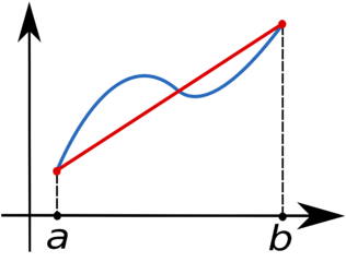
$$ \int_{a}^{b}f(x)dx $$

we can partition the integration interval $[a,b]$ into smaller subintervals, and approximate the area under the curve for each subinterval by the area of the trapezoid created by linearly interpolating between the two function values at each end of the subinterval:

The blue line represents the function $f(x)$ and the red line is the linear interpolation. By subdividing the interval $[a,b]$, the area under $f(x)$ can thus be approximated as the sum of the areas of all the resulting trapezoids.

If we denote by $x_{i}$ ($i=0,\ldots,n,$ with $x_{0}=a$ and $x_{n}=b$) the abscissas where the function is sampled, then

$$ \int_{a}^{b}f(x)dx\approx\frac{1}{2}\sum_{i=1}^{n}\left(x_{i}-x_{i-1}\right)\left(f(x_{i})+f(x_{i-1})\right). $$

The common case of using equally spaced abscissas with spacing $h=(b-a)/n$ reads simply

$$ \int_{a}^{b}f(x)dx\approx\frac{h}{2}\sum_{i=1}^{n}\left(f(x_{i})+f(x_{i-1})\right). $$

One frequently receives the function values already precomputed, $y_{i}=f(x_{i}),$ so the equation above becomes

$$ \int_{a}^{b}f(x)dx\approx\frac{1}{2}\sum_{i=1}^{n}\left(x_{i}-x_{i-1}\right)\left(y_{i}+y_{i-1}\right). $$

Let's first preload the necessary libraries

In [2]:

%matplotlib inline
import numpy as np
import matplotlib.pyplot as plt

Exercises¶

1¶

Write a function trapz(x, y), that applies the trapezoid formula to pre-computed values, where x and y are 1-d arrays.

In [3]:

def trapz(x, y):
    return 0.5*np.sum((x[1:]-x[:-1])*(y[1:]+y[:-1]))

2¶

Write a function trapzf(f, a, b, npts=100) that accepts a function f, the endpoints a and b and the number of samples to take npts. Sample the function uniformly at these points and return the value of the integral.

In [4]:

def trapzf(f, a, b, npts=100):
    x = np.linspace(a, b, npts)
    y = f(x)
    return trapz(x, y)

3¶

Verify that both functions above are correct by showing that they produces correct values for a simple integral such as $\int_0^3 x^2$.

In [6]:

exact = 9.0
x = np.linspace(0, 3, 50)
y = x**2

print(exact)
print(trapz(x, y))

def f(x): return x**2
print(trapzf(f, 0, 3, 50))

9.0
9.00187421908
9.00187421908

4¶

Repeat the integration for several values of npts, and plot the error as a function of npts for the integral in #3.

In [7]:

npts = [5, 10, 20, 50, 100, 200]
err = []
for n in npts:
    err.append(trapzf(f, 0, 3, n)-exact)

In [9]:

plt.semilogy(npts, np.abs(err))
plt.title(r'Trapezoid approximation to $\int_0^3 x^2$')
plt.xlabel('npts')
plt.ylabel('Error');

An illustration using matplotlib and scipy¶

We define a function with a little more complex look

In [10]:

def f(x):
    return (x-3)*(x-5)*(x-7)+85

x = np.linspace(0, 10, 200)
y = f(x)

Choose a region to integrate over and take only a few points in that region

In [11]:

a, b = 1, 9
xint = x[logical_and(x>=a, x<=b)][::30]
yint = y[logical_and(x>=a, x<=b)][::30]

Plot both the function and the area below it in the trapezoid approximation

In [12]:

plt.plot(x, y, lw=2)
plt.axis([0, 10, 0, 140])
plt.fill_between(xint, 0, yint, facecolor='gray', alpha=0.4)
plt.text(0.5 * (a + b), 30,r"$\int_a^b f(x)dx$", horizontalalignment='center', fontsize=20);

In practice, we don't need to implement numerical integration ourselves, as scipy has both basic trapezoid rule integrators and more sophisticated ones. Here we illustrate both:

In [14]:

from scipy.integrate import quad, trapz
integral, error = quad(f, 1, 9)
print("The integral is:", integral, "+/-", error)
print("The trapezoid approximation with", len(xint), "points is:", trapz(yint, xint))

The integral is: 680.0 +/- 7.549516567451064e-12
The trapezoid approximation with 6 points is: 621.286411141