9. PageRank with Eigen Decompositions¶

Two Handy Tricks¶

Here are two tools that we'll be using today, which are useful in general.

1. Psutil is a great way to check on your memory usage. This will be useful here since we are using a larger data set.

In [462]:

import psutil

In [447]:

process = psutil.Process(os.getpid())
t = process.memory_info()

In [449]:

t.vms, t.rss

Out[449]:

(19475513344, 17856520192)

In [450]:

def mem_usage():
    process = psutil.Process(os.getpid())
    return process.memory_info().rss / psutil.virtual_memory().total

In [451]:

mem_usage()

Out[451]:

0.13217061955758594

2. TQDM gives you progress bars.

In [364]:

from time import sleep

In [463]:

# Without TQDM
s = 0
for i in range(10):
    s += i
    sleep(0.2)
print(s)

In [465]:

# With TQDM
from tqdm import tqdm

s = 0
for i in tqdm(range(10)):
    s += i
    sleep(0.2)
print(s)

100%|██████████| 10/10 [00:02<00:00,  4.96it/s]

Motivation¶

Review

What is SVD?
What are some applications of SVD?

Additional SVD Application¶

An interesting use of SVD that I recently came across was as a step in the de-biasing of Word2Vec word embeddings, from Quantifying and Reducing Stereotypes in Word Embeddings(Bolukbasi, et al).

Word2Vec is a useful library released by Google that represents words as vectors. The similarity of vectors captures semantic meaning, and analogies can be found, such as Paris:France :: Tokyo: Japan.

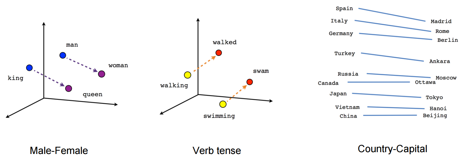(source: [Vector Representations of Words](https://www.tensorflow.org/versions/r0.10/tutorials/word2vec/))

However, these embeddings can implicitly encode bias, such as father:doctor :: mother:nurse and man:computer programmer :: woman:homemaker.

One approach for de-biasing the space involves using SVD to reduce the dimensionality (Bolukbasi paper).

You can read more about bias in word embeddings:

How Vector Space Mathematics Reveals the Hidden Sexism in Language(MIT Tech Review)
ConceptNet: better, less-stereotyped word vectors
Semantics derived automatically from language corpora necessarily contain human biases (excellent and very interesting paper!)

Ways to think about SVD¶

Data compression
SVD trades a large number of features for a smaller set of better features
All matrices are diagonal (if you use change of bases on the domain and range)

Perspectives on SVD¶

We usually talk about SVD in terms of matrices, $$A = U \Sigma V^T$$ but we can also think about it in terms of vectors. SVD gives us sets of orthonormal vectors ${v_j}$ and ${u_j}$ such that $$ A v_j = \sigma_j u_j $$

$\sigma_j$ are scalars, called singular values

Q: Does this remind you of anything?

Answer¶

Relationship between SVD and Eigen Decomposition: the left-singular vectors of A are the eigenvectors of $AA^T$. The right-singular vectors of A are the eigenvectors of $A^T A$. The non-zero singular values of A are the square roots of the eigenvalues of $A^T A$ (and $A A^T$).

SVD is a generalization of eigen decomposition. Not all matrices have eigen values, but ALL matrices have singular values.

Let's forget SVD for a bit and talk about how to find the eigenvalues of a symmetric positive definite matrix...

Further resources on SVD¶

Today: Eigen Decomposition¶

The best classical methods for computing the SVD are variants on methods for computing eigenvalues. In addition to their links to SVD, Eigen decompositions are useful on their own as well. Here are a few practical applications of eigen decomposition:

rapid matrix powers
nth Fibonacci number
Behavior of ODEs
Markov Chains (health care economics, Page Rank)
Linear Discriminant Analysis on Iris dataset

Check out the 3 Blue 1 Brown videos on Change of basis and Eigenvalues and eigenvectors

"Eigenvalues are a way to see into the heart of a matrix... All the difficulties of matrices are swept away" -Strang

Vocab: A Hermitian matrix is one that is equal to it's own conjugate transpose. In the case of real-valued matrices (which is all we are considering in this course), Hermitian means the same as Symmetric.

Relevant Theorems:

If A is symmetric, then eigenvalues of A are real and $A = Q \Lambda Q^T$
If A is triangular, then its eigenvalues are equal to its diagonal entries

DBpedia Dataset¶

Let's start with the Power Method, which finds one eigenvector. What good is just one eigenvector? you may be wondering. This is actually the basis for PageRank (read The $25,000,000,000 Eigenvector: the Linear Algebra Behind Google for more info)

Instead of trying to rank the importance of all websites on the internet, we are going to use a dataset of Wikipedia links from DBpedia. DBpedia provides structured Wikipedia data available in 125 languages.

"The full DBpedia data set features 38 million labels and abstracts in 125 different languages, 25.2 million links to images and 29.8 million links to external web pages; 80.9 million links to Wikipedia categories, and 41.2 million links to YAGO categories" --about DBpedia

Today's lesson is inspired by this SciKit Learn Example

Imports¶

In [361]:

import os, numpy as np, pickle
from bz2 import BZ2File
from datetime import datetime
from pprint import pprint
from time import time
from tqdm import tqdm_notebook
from scipy import sparse

from sklearn.decomposition import randomized_svd
from sklearn.externals.joblib import Memory
from urllib.request import urlopen

Downloading the data¶

The data we have are:

redirects: URLs that redirect to other URLs
links: which pages link to which other pages

Note: this takes a while

In [367]:

PATH = 'data/dbpedia/'
URL_BASE = 'http://downloads.dbpedia.org/3.5.1/en/'
filenames = ["redirects_en.nt.bz2", "page_links_en.nt.bz2"]

for filename in filenames:
    if not os.path.exists(PATH+filename):
        print("Downloading '%s', please wait..." % filename)
        open(PATH+filename, 'wb').write(urlopen(URL_BASE+filename).read())

In [368]:

redirects_filename = PATH+filenames[0]
page_links_filename = PATH+filenames[1]

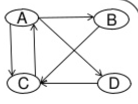
Graph Adjacency Matrix¶

We will construct a graph adjacency matrix, of which pages point to which.

(source: [PageRank and HyperLink Induced Topic Search](https://www.slideshare.net/priyabrata232/page-rank-and-hyperlink))

The power $A^2$ will give you how many ways there are to get from one page to another in 2 steps. You can see a more detailed example, as applied to airline travel, worked out in these notes.

We want to keep track of which pages point to which pages. We will store this in a square matrix, with a $1$ in position $(r, c)$ indicating that the topic in row $r$ points to the topic in column $c$

You can read more about graphs here.

Data Format¶

One line of the file looks like:

<http://dbpedia.org/resource/AfghanistanHistory> <http://dbpedia.org/property/redirect> <http://dbpedia.org/resource/History_of_Afghanistan> .

In the below slice, the plus 1, -1 are to remove the <>

In [369]:

DBPEDIA_RESOURCE_PREFIX_LEN = len("http://dbpedia.org/resource/")
SLICE = slice(DBPEDIA_RESOURCE_PREFIX_LEN + 1, -1)

In [370]:

def get_lines(filename): return (line.split() for line in BZ2File(filename))

Loop through redirections and create dictionary of source to final destination

In [371]:

def get_redirect(targ, redirects):
    seen = set()
    while True:
        transitive_targ = targ
        targ = redirects.get(targ)
        if targ is None or targ in seen: break
        seen.add(targ)
    return transitive_targ

In [372]:

def get_redirects(redirects_filename):
    redirects={}
    lines = get_lines(redirects_filename)
    return {src[SLICE]:get_redirect(targ[SLICE], redirects) 
                for src,_,targ,_ in tqdm_notebook(lines, leave=False)}

In [373]:

redirects = get_redirects(redirects_filename)

In [374]:

mem_usage()

Out[374]:

13.766303744

In [375]:

def add_item(lst, redirects, index_map, item):
    k = item[SLICE]
    lst.append(index_map.setdefault(redirects.get(k, k), len(index_map)))

In [376]:

limit=119077682 #5000000

In [377]:

# Computing the integer index map
index_map = dict() # links->IDs
lines = get_lines(page_links_filename)
source, destination, data = [],[],[]
for l, split in tqdm_notebook(enumerate(lines), total=limit):
    if l >= limit: break
    add_item(source, redirects, index_map, split[0])
    add_item(destination, redirects, index_map, split[2])
    data.append(1)

In [379]:

n=len(data); n

Out[379]:

119077682

Looking at our data¶

The below steps are just to illustrate what info is in our data and how it is structured. They are not efficient.

Let's see what type of items are in index_map:

In [425]:

index_map.popitem()

Out[425]:

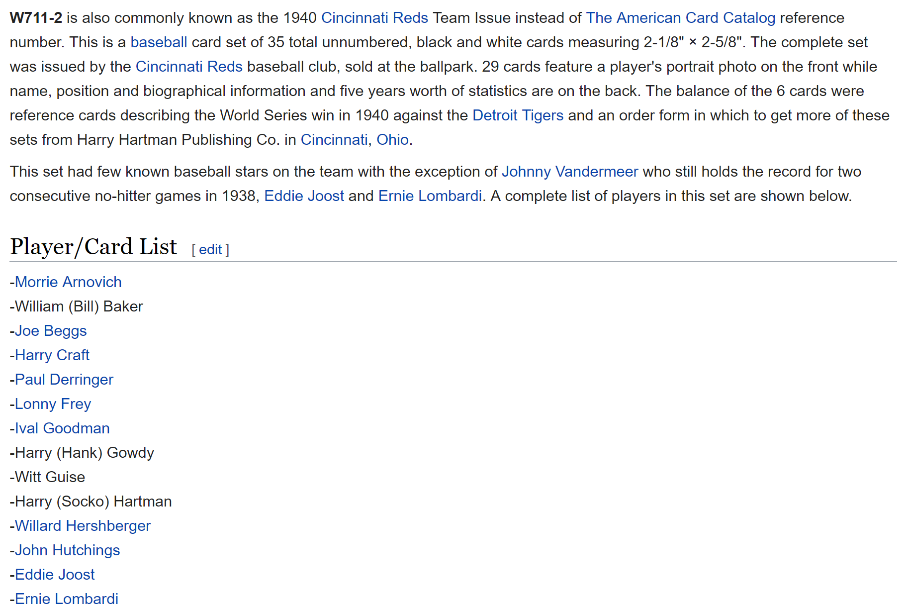
(b'1940_Cincinnati_Reds_Team_Issue', 9991173)

Let's look at one item in our index map:

1940_Cincinnati_Reds_Team_Issue has index $9991173$. This only shows up once in the destination list:

In [427]:

[i for i,x in enumerate(source) if x == 9991173]

Out[427]:

[119077649]

In [428]:

source[119077649], destination[119077649]

Out[428]:

(9991173, 9991050)

Now, we want to check which page is the source (has index $9991050$). Note: usually you should not access a dictionary by searching for its values. This is inefficient and not how dictionaries are intended to be used.

In [429]:

for page_name, index in index_map.items():
    if index == 9991050:
        print(page_name)

b'W711-2'

We can see on Wikipedia that the Cincinati Red Teams Issue has redirected to W711-2:

In [431]:

test_inds = [i for i,x in enumerate(source) if x == 9991050]

In [466]:

len(test_inds)

Out[466]:

In [433]:

test_inds[:5]

Out[433]:

[119076756, 119076757, 119076758, 119076759, 119076760]

In [434]:

test_dests = [destination[i] for i in test_inds]

Now, we want to check which page is the source (has index 9991174):

In [435]:

for page_name, index in index_map.items():
    if index in test_dests:
        print(page_name)

b'Baseball'
b'Ohio'
b'Cincinnati'
b'Flash_Thompson'
b'1940'
b'1938'
b'Lonny_Frey'
b'Cincinnati_Reds'
b'Ernie_Lombardi'
b'Baseball_card'
b'James_Wilson'
b'Trading_card'
b'Detroit_Tigers'
b'Baseball_culture'
b'Frank_McCormick'
b'Bucky_Walters'
b'1940_World_Series'
b'Billy_Werber'
b'Ival_Goodman'
b'Harry_Craft'
b'Paul_Derringer'
b'Johnny_Vander_Meer'
b'Cigarette_card'
b'Eddie_Joost'
b'Myron_McCormick'
b'Beckett_Media'
b'Icarus_affair'
b'Ephemera'
b'Sports_card'
b'James_Turner'
b'Jimmy_Ripple'
b'Lewis_Riggs'
b'The_American_Card_Catalog'
b'Rookie_card'
b'Willard_Hershberger'
b'Elmer_Riddle'
b'Joseph_Beggs'
b'Witt_Guise'
b'Milburn_Shoffner'

We can see that the items in the list appear in the wikipedia page:

(Source: [Wikipedia](https://en.wikipedia.org/wiki/W711-2))

Create Matrix¶

Below we create a sparse matrix using Scipy's COO format, and that convert it to CSR.

Questions: What are COO and CSR? Why would we create it with COO and then convert it right away?

In [341]:

X = sparse.coo_matrix((data, (destination,source)), shape=(n,n), dtype=np.float32)
X = X.tocsr()

In [347]:

del(data,destination, source)

In [342]:

Out[342]:

<119077682x119077682 sparse matrix of type '<class 'numpy.float32'>'
	with 93985520 stored elements in Compressed Sparse Row format>

In [343]:

names = {i: name for name, i in index_map.items()}

In [349]:

mem_usage()

Out[349]:

12.903882752

Save matrix so we don't have to recompute¶

In [350]:

pickle.dump(X, open(PATH+'X.pkl', 'wb'))
pickle.dump(index_map, open(PATH+'index_map.pkl', 'wb'))

In [316]:

X = pickle.load(open(PATH+'X.pkl', 'rb'))
index_map = pickle.load(open(PATH+'index_map.pkl', 'rb'))

In [317]:

names = {i: name for name, i in index_map.items()}

In [351]:

Out[351]:

<119077682x119077682 sparse matrix of type '<class 'numpy.float32'>'
	with 93985520 stored elements in Compressed Sparse Row format>

Power method¶

Motivation¶

An $n \times n$ matrix $A$ is diagonalizable if it has $n$ linearly independent eigenvectors $v_1,\, \ldots v_n$.

Then any $w$ can be expressed $w = \sum_{j=1}^n c_j v_j $, for some scalars $c_j$.

Exercise: Show that $$ A^k w = \sum_{j=1}^n c_j \lambda_j^k v_j$$

Question: How will this behave for large $k$?

This is inspiration for the power method.

Code¶

In [281]:

def show_ex(v):
    print(', '.join(names[i].decode() for i in np.abs(v.squeeze()).argsort()[-1:-10:-1]))

In [453]:

?np.squeeze

How to normalize a sparse matrix:

In [336]:

S = sparse.csr_matrix(np.array([[1,2],[3,4]]))
Sr = S.sum(axis=0).A1; Sr

Out[336]:

array([4, 6], dtype=int64)

numpy.matrix.A1

In [337]:

S.indices

Out[337]:

array([0, 1, 0, 1], dtype=int32)

In [338]:

S.data

Out[338]:

array([1, 2, 3, 4], dtype=int64)

In [339]:

S.data / np.take(Sr, S.indices)

Out[339]:

array([ 0.25   ,  0.33333,  0.75   ,  0.66667])

In [328]:

def power_method(A, max_iter=100):
    n = A.shape[1]
    A = np.copy(A)
    A.data /= np.take(A.sum(axis=0).A1, A.indices)

    scores = np.ones(n, dtype=np.float32) * np.sqrt(A.sum()/(n*n)) # initial guess
    for i in range(max_iter):
        scores = A @ scores
        nrm = np.linalg.norm(scores)
        scores /= nrm
        print(nrm)

    return scores

Question: Why normalize the scores on each iteration?

In [345]:

scores = power_method(X, max_iter=10)

In [346]:

show_ex(scores)

Living_people, Year_of_birth_missing_%28living_people%29, United_States, United_Kingdom, Race_and_ethnicity_in_the_United_States_Census, France, Year_of_birth_missing, World_War_II, Germany

In [ ]:

In [327]:

mem_usage()

Out[327]:

11.692331008

Comments¶

Many advanced eigenvalue algorithms that are used in practice are variations on the power method.

In Lesson 3: Background Removal, we used Facebook's fast randomized pca/svd library, fbpca. Check out the source code for the pca method we used. It uses the power method!

Further Study

Check out Google Page Rank, Power Iteration and the Second EigenValue of the Google Matrix for animations of the distribution as it converges.
The convergence rate of the power method is the ratio of the largest eigenvalue to the 2nd largest eigenvalue. It can be speeded up by adding shifts. To find eigenvalues other than the largest, a method called deflation can be used. See Chapter 12.1 of Greenbaum & Chartier for more details.
Krylov Subspaces: In the Power Iteration, notice that we multiply by our matrix A each time, effectively calculating $$Ab,\,A^2b,\,A^3b,\,A^4b\, \ldots$$

The matrix with those vectors as columns is called the Krylov matrix, and the space spanned by those vectors is the Krylov subspace. Keep this in mind for later.

Compare to SVD¶

In [27]:

%time U, s, V = randomized_svd(X, 3, n_iter=3)

CPU times: user 8min 40s, sys: 1min 20s, total: 10min 1s
Wall time: 5min 56s

In [28]:

mem_usage()

Out[28]:

28.353073152

In [30]:

# Top wikipedia pages according to principal singular vectors
show_ex(U.T[0])

List_of_World_War_II_air_aces, List_of_animated_feature-length_films, List_of_animated_feature_films:2000s, International_Swimming_Hall_of_Fame, List_of_museum_ships, List_of_linguists, List_of_television_programs_by_episode_count, List_of_game_show_hosts, List_of_astronomers

In [31]:

show_ex(U.T[1])

List_of_former_United_States_senators, List_of_United_States_Representatives_from_New_York, List_of_United_States_Representatives_from_Pennsylvania, Members_of_the_110th_United_States_Congress, List_of_Justices_of_the_Ohio_Supreme_Court, Congressional_endorsements_for_the_2008_United_States_presidential_election, List_of_United_States_Representatives_in_the_110th_Congress_by_seniority, List_of_Members_of_the_United_States_House_of_Representatives_in_the_103rd_Congress_by_seniority, List_of_United_States_Representatives_in_the_111th_Congress_by_seniority

In [32]:

show_ex(V[0])

United_States, Japan, United_Kingdom, Germany, Race_and_ethnicity_in_the_United_States_Census, France, United_States_Army_Air_Forces, Australia, Canada

In [33]:

show_ex(V[1])

Democratic_Party_%28United_States%29, Republican_Party_%28United_States%29, Democratic-Republican_Party, United_States, Whig_Party_%28United_States%29, Federalist_Party, National_Republican_Party, Catholic_Church, Jacksonian_democracy

Exercise: Normalize the data in various ways. Don't overwrite the adjacency matrix, but instead create a new one. See how your results differ.

Eigen Decomposition vs SVD:

SVD involves 2 bases, eigen decomposition involves 1 basis
SVD bases are orthonormal, eigen basis generally not orthogonal
All matrices have an SVD, not all matrices (not even all square) have an eigen decomposition

QR Algorithm¶

We used the power method to find the eigenvector corresponding to the largest eigenvalue of our matrix of Wikipedia links. This eigenvector gave us the relative importance of each Wikipedia page (like a simplified PageRank).

Next, let's look at a method for finding all eigenvalues of a symmetric, positive definite matrix. This method includes 2 fundamental algorithms in numerical linear algebra, and is a basis for many more complex methods.

The Second Eigenvalue of the Google Matrix: has "implications for the convergence rate of the standard PageRank algorithm as the web scales, for the stability of PageRank to perturbations to the link structure of the web, for the detection of Google spammers, and for the design of algorithms to speed up PageRank".

Avoiding Confusion: QR Algorithm vs QR Decomposition¶

The QR algorithm uses something called the QR decomposition. Both are important, so don't get them confused. The QR decomposition decomposes a matrix $A = QR$ into a set of orthonormal columns $Q$ and a triangular matrix $R$. We will look at several ways to calculate the QR decomposition in a future lesson. For now, just know that it is giving us an orthogonal matrix and a triangular matrix.

Linear Algebra¶

Two matrices $A$ and $B$ are similar if there exists a non-singular matrix $X$ such that $$B = X^{-1}AX$$

Watch this: Change of Basis

Theorem: If $X$ is non-singular, then $A$ and $X^{-1}AX$ have the same eigenvalues.

More Linear Algebra¶

A Schur factorization of a matrix $A$ is a factorization: $$ A = Q T Q^*$$ where $Q$ is unitary and $T$ is upper-triangular.

Question: What can you say about the eigenvalues of $A$?

Theorem: Every square matrix has a Schur factorization.

Other resources¶

Review: Linear combinations, span, and basis vectors

See Lecture 24 for proofs of above theorems (and more!)

Algorithm¶

The most basic version of the QR algorithm:

for k=1,2,...
    Q, R = A
    A = R @ Q

Under suitable assumptions, this algorithm converges to the Schur form of A!

Why it works¶

Written again, only with subscripts:

$A_0 = A$

for $k=1,2,\ldots$

$\quad Q_k$, $R_k$ = $A_{k-1}$

$\quad A_k$ = $R_k Q_k$

We can think of this as constructing sequences of $A_k$, $Q_k$, and $R_k$.

$$ A_k = Q_k \, R_k $$$$ Q_k^{-1} \, A_k = R_k$$

Thus,

$$ R_k Q_k = Q_k^{-1} \, A_k \, Q_k $$$$A_k = Q_k^{-1} \ldots Q_2^{-1} Q_1^{-1} A Q_1 Q_2 \dots Q_k$$

Trefethen proves the following on page 216-217:

$$A^k = Q_1 Q_2 \dots Q_k R_k R_{k-1}\dots R_1$$

Key: The QR algorithm constructs orthonormal bases for successive powers $A^k$. And remember the close relationship between powers of A and the eigen decomposition.

To learn more, read up on Rayleigh quotients.

Pure QR¶

In [467]:

n = 6
A = np.random.rand(n,n)
AT = A @ A.T

In [477]:

def pure_qr(A, max_iter=1000):
    Ak = np.copy(A)
    n = A.shape[0]
    QQ = np.eye(n)
    for k in range(max_iter):
        Q, R = np.linalg.qr(Ak)
        Ak = R @ Q
        QQ = QQ @ Q
        if k % 100 == 0:
            print(Ak)
            print("\n")
    return Ak, QQ

Pure QR¶

In [479]:

Out[479]:

array([[ 0.62878,  0.23258,  0.63909,  0.90223,  0.94772,  0.80247],
       [ 0.64361,  0.52469,  0.92231,  0.32869,  0.58532,  0.75104],
       [ 0.44363,  0.00427,  0.62418,  0.47093,  0.6762 ,  0.28078],
       [ 0.14629,  0.76324,  0.23316,  0.55208,  0.21712,  0.20255],
       [ 0.56122,  0.08282,  0.12788,  0.10419,  0.40358,  0.69272],
       [ 0.41172,  0.06411,  0.92162,  0.53139,  0.27901,  0.61592]])

In [478]:

Ak, Q = pure_qr(A)

[[ 2.65646  0.21386  0.16765  0.75256  0.61251  0.93518]
 [ 0.52744  0.47579  0.17052 -0.41086 -0.21182 -0.01876]
 [ 0.29923  0.06964  0.11173  0.1879  -0.29101  0.60032]
 [ 0.2274   0.46162 -0.26654  0.08899  0.24631  0.26447]
 [-0.06093  0.02892  0.34162  0.07533  0.02393 -0.05456]
 [-0.06025  0.02694 -0.11675 -0.00927 -0.11939 -0.00767]]


[[ 2.78023  0.52642  0.0395  -0.11135  0.1569   1.15184]
 [ 0.       0.18624 -0.297   -0.07256 -0.04537  0.27907]
 [ 0.       0.69328  0.34105 -0.12198  0.11029  0.0992 ]
 [-0.      -0.0494  -0.02057  0.09461  0.59466  0.09115]
 [-0.       0.00008 -0.02659 -0.40372  0.06542  0.38612]
 [-0.       0.       0.       0.      -0.      -0.11832]]


[[ 2.78023 -0.12185 -0.51401  0.17625 -0.07467  1.15184]
 [ 0.       0.2117  -0.70351  0.09974 -0.02986  0.00172]
 [ 0.       0.28284  0.32635 -0.0847  -0.08488 -0.29104]
 [-0.      -0.00068 -0.00088 -0.01282  0.54836  0.13447]
 [-0.       0.      -0.00102 -0.45718  0.16208 -0.37726]
 [-0.       0.       0.       0.      -0.      -0.11832]]


[[ 2.78023 -0.33997  0.4049   0.17949  0.06291  1.15184]
 [ 0.       0.48719 -0.48788 -0.05831 -0.12286 -0.23486]
 [ 0.       0.49874  0.05104 -0.07191  0.03638  0.17261]
 [ 0.       0.00002  0.       0.02128  0.41958  0.3531 ]
 [ 0.      -0.       0.00002 -0.58571  0.1278  -0.18838]
 [ 0.       0.       0.      -0.       0.      -0.11832]]


[[ 2.78023  0.35761  0.38941  0.07462  0.17493  1.15184]
 [ 0.       0.0597  -0.55441 -0.0681  -0.04456  0.14084]
 [ 0.       0.43221  0.47853 -0.06068  0.12117  0.25519]
 [-0.      -0.      -0.       0.16206  0.45708  0.37724]
 [-0.       0.      -0.      -0.54821 -0.01298  0.1336 ]
 [ 0.       0.       0.       0.      -0.      -0.11832]]


[[ 2.78023  0.06853 -0.52424  0.05224 -0.18287  1.15184]
 [ 0.       0.36572 -0.6889   0.07864 -0.09263  0.105  ]
 [ 0.       0.29772  0.17251 -0.09836 -0.02347 -0.27191]
 [ 0.      -0.      -0.       0.13719  0.57888 -0.20884]
 [ 0.       0.      -0.      -0.42642  0.01189 -0.34139]
 [ 0.       0.       0.       0.      -0.      -0.11832]]


[[ 2.78023 -0.52782  0.03045 -0.14389 -0.12436  1.15184]
 [ 0.       0.25091 -0.27593  0.08994 -0.06581 -0.28672]
 [ 0.       0.7107   0.28732  0.10154  0.04751 -0.05245]
 [ 0.      -0.      -0.       0.0297  -0.59054 -0.01234]
 [ 0.      -0.       0.       0.41475  0.11938 -0.40001]
 [ 0.       0.       0.       0.       0.      -0.11832]]


[[ 2.78023  0.1533   0.50599  0.18983  0.01158  1.15184]
 [ 0.       0.18627 -0.69511 -0.0991  -0.00189  0.01621]
 [ 0.       0.29151  0.35196  0.05638 -0.10949  0.29102]
 [ 0.      -0.      -0.      -0.02207 -0.48261  0.25246]
 [ 0.      -0.       0.       0.52268  0.17116  0.31053]
 [ 0.       0.       0.       0.       0.      -0.11832]]


[[ 2.78023  0.29683 -0.43751 -0.13852  0.13032  1.15184]
 [ 0.       0.48375 -0.53231 -0.01164  0.13482  0.216  ]
 [ 0.       0.45431  0.05448 -0.07972 -0.01795 -0.19571]
 [ 0.      -0.       0.       0.10042 -0.40743 -0.39915]
 [ 0.      -0.       0.       0.59786  0.04867 -0.02893]
 [ 0.       0.       0.       0.       0.      -0.11832]]


[[ 2.78023 -0.39373 -0.35284  0.00838 -0.19     1.15184]
 [ 0.       0.05184 -0.51278  0.05752 -0.0564  -0.16496]
 [ 0.       0.47384  0.48639  0.09426  0.09806 -0.24031]
 [ 0.      -0.      -0.       0.17043 -0.52593  0.30622]
 [ 0.      -0.       0.       0.47936 -0.02134 -0.25766]
 [ 0.       0.       0.       0.       0.      -0.11832]]

Let's compare to the eigenvalues:

In [469]:

np.linalg.eigvals(A)

Out[469]:

array([ 2.78023+0.j     , -0.11832+0.j     ,  0.26911+0.44246j,
        0.26911-0.44246j,  0.07454+0.49287j,  0.07454-0.49287j])

Check that Q is orthogonal:

In [476]:

np.allclose(np.eye(n), Q @ Q.T), np.allclose(np.eye(n), Q.T @ Q)

Out[476]:

(True, True)

This is really really slow.

Practical QR (QR with shifts)¶

Idea: Instead of factoring $A_k$ as $Q_k R_k$,

Get the QR factorization $$A_k - s_k I = Q_k R_k$$
Set $$A_{k+1} = R_k Q_k + s_k I$$

Choose $s_k$ to approximate an eigenvalue of $A$. We'll use $s_k = A_k(m,m)$.

The idea of adding shifts to speed up convergence shows up in many algorithms in numerical linear algebra (including the power method, inverse iteration, and Rayleigh quotient iteration).

Homework: Add shifts to the QR algorithm¶

In [460]:

#Exercise: Add shifts to the QR algorithm
#Exercise: def practical_qr(A, iters=10):
#Exercise:     return Ak, Q

Practical QR¶

In [204]:

Ak, Q = practical_qr(A, 10)

[ 5.16264  2.53603  0.31923  0.35315  0.97569  0.43615]
[ 7.99381  0.05922  0.34478  0.29482  0.79026  0.29999]
[ 8.00491  0.04358  0.89735  0.26386  0.26182  0.31135]
[ 8.00493  0.13648  0.91881  0.14839  0.24313  0.33115]
[ 8.00493  0.43377  0.62809  0.13429  0.24592  0.33589]
[ 8.00493  0.81058  0.25128  0.13297  0.24722  0.3359 ]
[ 8.00493  0.98945  0.07221  0.13292  0.24747  0.3359 ]
[ 8.00493  1.0366   0.02497  0.13296  0.24751  0.3359 ]
[ 8.00493  1.04688  0.01465  0.13299  0.24752  0.3359 ]
[ 8.00493  1.04902  0.0125   0.13301  0.24753  0.3359 ]

Check that Q is orthogonal:

In [201]:

np.allclose(np.eye(n), Q @ Q.T), np.allclose(np.eye(n), Q.T @ Q)

Out[201]:

(True, True)

Let's compare to the eigenvalues:

In [196]:

np.linalg.eigvals(A)

Out[196]:

array([ 2.68500+0.j     ,  0.19274+0.41647j,  0.19274-0.41647j,
       -0.35988+0.43753j, -0.35988-0.43753j, -0.18346+0.j     ])

Problem: This is better than the unshifted version (which wasn't even guaranteed to converge), but is still really slow! In fact, it is $\mathcal{O}(n^4)$, which is awful.

In the case of symmetric matrices, it's $\mathcal{O}(n^3)$

However, if you start with a Hessenberg matrix (zeros below the first subdiagonal), it's faster: $\mathcal{O}(n^3)$, and $\mathcal{O}(n^2)$ if symmetric.

A Two-Phase Approach¶

In practice, a two phase approach is used to find eigenvalues:

Reduce the matrix to Hessenberg form (zeros below the first subdiagonal)
Iterative process that causes Hessenberg to converge to a triangular matrix. The eigenvalues of a triangular matrix are the values on the diagonal, so we are finished!

(source: Trefethen, Lecture 25)

In the case of a Hermitian matrix, this approach is even faster, since the intermediate step is also Hermitian (and a Hermitian Hessenberg is tridiagonal).

(source: Trefethen, Lecture 25)

Phase 1 reaches an exact solution in a finite number of steps, whereas Phase 2 theoretically never reaches the exact solution.

We've already done step 2: the QR algorithm. Remember that it would be possible to just use the QR algorithm, but ridiculously slow.

Arnoldi Iteration¶

We can use the Arnoldi iteration for phase 1 (and the QR algorithm for phase 2).

Initializations¶

In [459]:

import numpy as np
n = 5
A0 = np.random.rand(n,n)  #.astype(np.float64)
A = A0 @ A0.T

np.set_printoptions(precision=5, suppress=True)

Linear Algebra Review: Projections¶

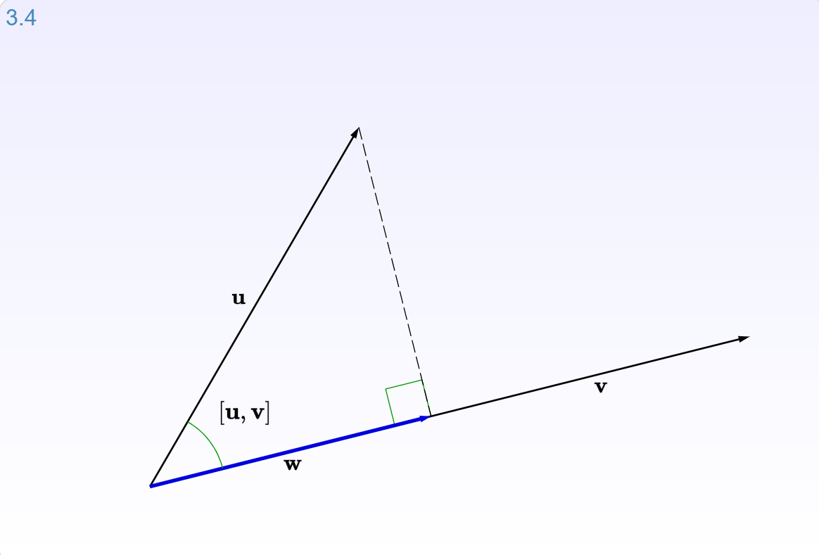
When vector $\mathbf{b}$ is projected onto a line $\mathbf{a}$, its projection $\mathbf{p}$ is the part of $\mathbf{b}$ along that line $\mathbf{a}$.

Let's look at interactive graphic (3.4) for section 3.2.2: Projections of the Immersive Linear Algebra online book.

(source: [Immersive Math](http://immersivemath.com/ila/ch03_dotproduct/ch03.html))

And here is what it looks like to project a vector onto a plane:

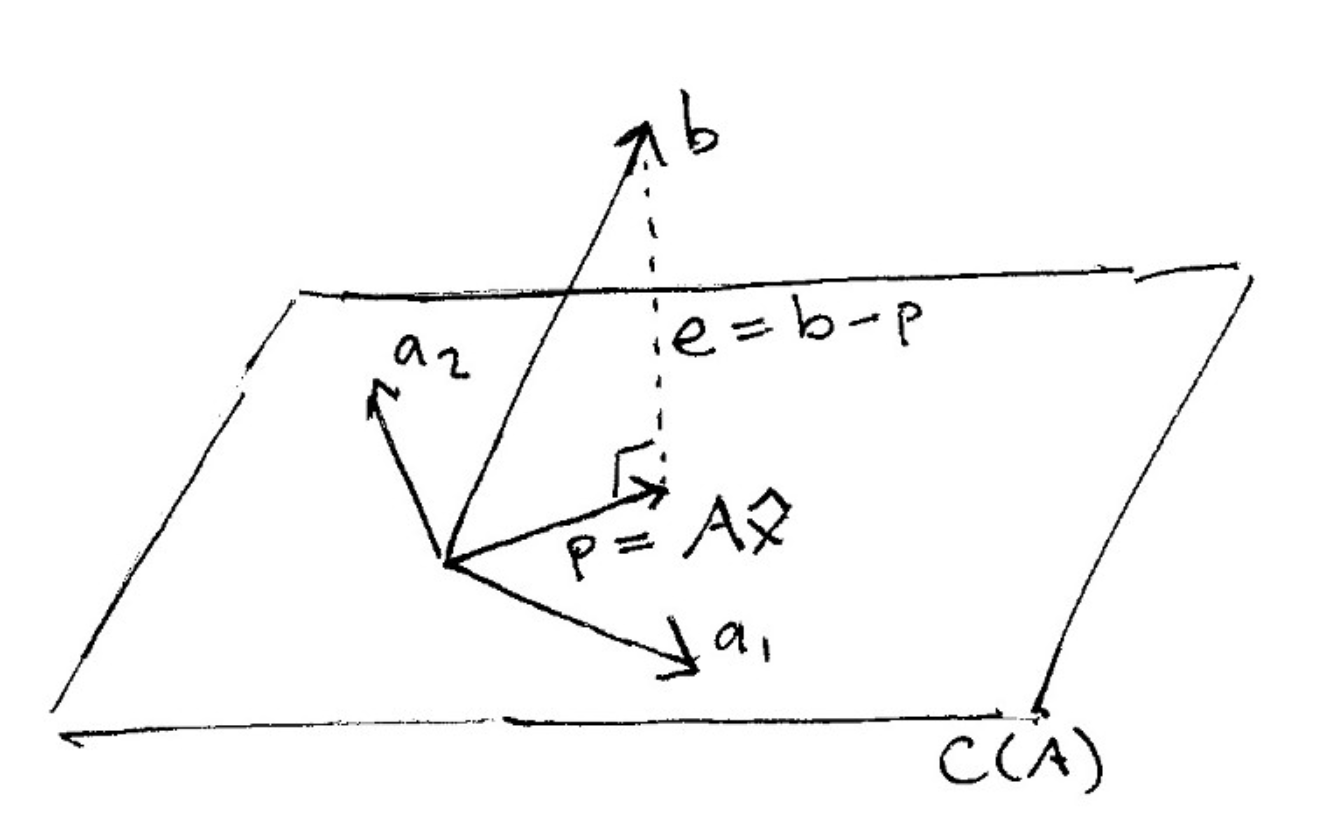(source: [The Linear Algebra View of Least-Squares Regression](https://medium.com/@andrew.chamberlain/the-linear-algebra-view-of-least-squares-regression-f67044b7f39b))

When vector $\mathbf{b}$ is projected onto a line $\mathbf{a}$, its projection $\mathbf{p}$ is the part of $\mathbf{b}$ along that line $\mathbf{a}$. So $\mathbf{p}$ is some multiple of $\mathbf{a}$. Let $\mathbf{p} = \hat{x}\mathbf{a}$ where $\hat{x}$ is a scalar.

Orthogonality¶

The key to projection is orthogonality: The line from $\mathbf{b}$ to $\mathbf{p}$ (which can be written $\mathbf{b} - \hat{x}\mathbf{a}$) is perpendicular to $\mathbf{a}$.

This means that $$ \mathbf{a} \cdot (\mathbf{b} - \hat{x}\mathbf{a}) = 0 $$

and so $$\hat{x} = \frac{\mathbf{a} \cdot \mathbf{b}}{\mathbf{a} \cdot \mathbf{a}} $$

The Algorithm¶

Motivation:

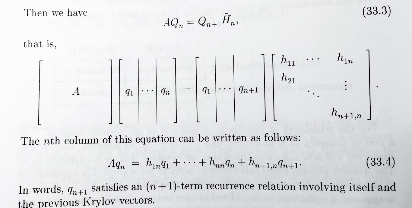
We want orthonormal columns in $Q$ and a Hessenberg $H$ such that $A Q = Q H$.

Thinking about it iteratively, $$ A Q_n = Q_{n+1} H_n $$ where $Q_{n+1}$ is $n\times n+1$ and $H_n$ is $n+1 \times n$. This creates a solvable recurrence relation.

(source: Trefethen, Lecture 33)

Pseudo-code for Arnoldi Algorithm

Start with an arbitrary vector (normalized to have norm 1) for first col of Q
for n=1,2,3...
    v = A @ nth col of Q
    for j=1,...n
        project v onto q_j, and subtract the projection off of v
        want to capture part of v that isn't already spanned by prev columns of Q
        store coefficients in H
    normalize v, and then make it the (n+1)th column of Q

Notice that we are multiplying A by the previous vector in Q and removing the components that are not orthogonal to the existing columns of Q.

Question: Repeated multiplications of A? Does this remind you of anything?

Answer:¶

In [ ]:

#Exercise Answer
The *Power Method* involved iterative multiplications by A as well!  

About how the Arnoldi Iteration works¶

With the Arnoldi Iteration, we are finding an orthonormal basis for the Krylov subspace.

The Krylov matrix $$ K = \left[b \; Ab \; A^2b \; \dots \; A^{n-1}b \right]$$ has a QR factorization $$K = QR$$ and that is the same $Q$ that is being found in the Arnoldi Iteration. Note that the Arnoldi Iteration does not explicity calculate $K$ or $R$.

Intuition: K contains good information about the largest eigenvalues of A, and the QR factorization reveals this information by peeling off one approximate eigenvector at a time.

The Arnoldi Iteration is two things:

the basis of many of the iterative algorithms of numerical linear algebra
a technique for finding eigenvalues of nonhermitian matrices

(Trefethen, page 257)

How Arnoldi Locates Eigenvalues

Carry out Arnoldi iteration
Periodically calculate the eigenvalues (called Arnoldi estimates or Ritz values) of the Hessenberg H, using the QR algorithm
Check at whether these values are converging. If they are, they're probably eigenvalues of A.

Implementation¶

In [246]:

# Decompose square matrix A @ Q ~= Q @ H
def arnoldi(A):
    m, n = A.shape
    assert(n <= m)
    
    # Hessenberg matrix
    H = np.zeros([n+1,n]) #, dtype=np.float64)
    # Orthonormal columns
    Q = np.zeros([m,n+1]) #, dtype=np.float64)
    # 1st col of Q is a random column with unit norm
    b = np.random.rand(m)
    Q[:,0] = b / np.linalg.norm(b)
    for j in range(n):
        v = A @ Q[:,j]
        for i in range(j+1):
            #This comes from the formula for projection of v onto q.
            #Since columns q are orthonormal, q dot q = 1
            H[i,j] = np.dot(Q[:,i], v)
            v = v - (H[i,j] * Q[:,i])
        H[j+1,j] = np.linalg.norm(v)
        Q[:,j+1] = v / H[j+1,j]
        
        # printing this to see convergence, would be slow to use in practice
        print(np.linalg.norm(A @ Q[:,:-1] - Q @ H))
    return Q[:,:-1], H[:-1,:]

In [86]:

Q, H = arnoldi(A)

8.59112969133
4.45398729097
0.935693639985
3.36613943339
0.817740180293

Check that H is tri-diagonal:

In [70]:

Out[70]:

array([[ 5.62746,  4.05085, -0.     ,  0.     , -0.     ],
       [ 4.05085,  3.07109,  0.33036,  0.     , -0.     ],
       [ 0.     ,  0.33036,  0.98297,  0.11172, -0.     ],
       [ 0.     ,  0.     ,  0.11172,  0.29777,  0.07923],
       [ 0.     ,  0.     ,  0.     ,  0.07923,  0.06034]])

Exercise¶

Write code to confirm that:

AQ = QH
Q is orthonormal

Answer:¶

In [71]:

#Exercise:

Out[71]:

True

In [456]:

#Exercise:

Out[456]:

True

General Case:¶

General Matrix: Now we can do this on our general matrix A (not symmetric). In this case, we are getting a Hessenberg instead of a Tri-diagonal

In [74]:

Q0, H0 = arnoldi(A0)

1.44287067354
1.06234006889
0.689291414367
0.918098818651
4.7124490411e-16

Check that H is Hessenberg:

In [76]:

H0

Out[76]:

array([[ 1.67416,  0.83233, -0.39284,  0.10833,  0.63853],
       [ 1.64571,  1.16678, -0.54779,  0.50529,  0.28515],
       [ 0.     ,  0.16654, -0.22314,  0.08577, -0.02334],
       [ 0.     ,  0.     ,  0.79017,  0.11732,  0.58978],
       [ 0.     ,  0.     ,  0.     ,  0.43238, -0.07413]])

In [77]:

np.allclose(A0 @ Q0, Q0 @ H0)

Out[77]:

True

In [78]:

np.allclose(np.eye(len(Q0)), Q0.T @ Q0), np.allclose(np.eye(len(Q0)), Q0 @ Q0.T)

Out[78]:

(True, True)

Putting it all together¶

In [215]:

def eigen(A, max_iter=20):
    Q, H = arnoldi(A)
    Ak, QQ = practical_qr(H, max_iter)
    U = Q @ QQ
    D = np.diag(Ak)
    return U, D

In [213]:

n = 10
A0 = np.random.rand(n,n)
A = A0 @ A0.T

In [242]:

U, D = eigen(A, 40)

14.897422908
1.57451192745
1.4820012435
0.668164424736
0.438450319682
0.674050723258
1.19470880942
0.217103444634
0.105443975462
3.8162597576e-15
[ 27.34799   1.22613   1.29671   0.70253   0.49651   0.56779   0.60974
   0.70123   0.19209   0.04905]
[ 27.34981   1.85544   1.04793   0.49607   0.44505   0.7106    1.00724
   0.07293   0.16058   0.04411]
[ 27.34981   2.01074   0.96045   0.54926   0.61117   0.8972    0.53424
   0.19564   0.03712   0.04414]
[ 27.34981   2.04342   0.94444   0.61517   0.89717   0.80888   0.25402
   0.19737   0.03535   0.04414]
[ 27.34981   2.04998   0.94362   0.72142   1.04674   0.58643   0.21495
   0.19735   0.03534   0.04414]
[ 27.34981   2.05129   0.94496   0.90506   0.95536   0.49632   0.21015
   0.19732   0.03534   0.04414]
[ 27.34981   2.05156   0.94657   1.09452   0.79382   0.46723   0.20948
   0.1973    0.03534   0.04414]
[ 27.34981   2.05161   0.94863   1.1919    0.70539   0.45628   0.20939
   0.19728   0.03534   0.04414]
[ 27.34981   2.05162   0.95178   1.22253   0.67616   0.45174   0.20939
   0.19727   0.03534   0.04414]
[ 27.34981   2.05162   0.95697   1.22715   0.66828   0.44981   0.2094
   0.19725   0.03534   0.04414]
[ 27.34981   2.05162   0.96563   1.22124   0.66635   0.44899   0.20941
   0.19724   0.03534   0.04414]
[ 27.34981   2.05162   0.97969   1.20796   0.66592   0.44864   0.20942
   0.19723   0.03534   0.04414]
[ 27.34981   2.05162   1.00135   1.18652   0.66585   0.44849   0.20943
   0.19722   0.03534   0.04414]
[ 27.34981   2.05162   1.03207   1.15586   0.66584   0.44843   0.20943
   0.19722   0.03534   0.04414]
[ 27.34981   2.05162   1.07082   1.11714   0.66584   0.4484    0.20944
   0.19721   0.03534   0.04414]
[ 27.34981   2.05162   1.11307   1.07489   0.66585   0.44839   0.20944
   0.1972    0.03534   0.04414]
[ 27.34981   2.05162   1.15241   1.03556   0.66585   0.44839   0.20945
   0.1972    0.03534   0.04414]
[ 27.34981   2.05162   1.18401   1.00396   0.66585   0.44839   0.20945
   0.1972    0.03534   0.04414]
[ 27.34981   2.05162   1.20652   0.98145   0.66585   0.44839   0.20946
   0.19719   0.03534   0.04414]
[ 27.34981   2.05162   1.22121   0.96676   0.66585   0.44839   0.20946
   0.19719   0.03534   0.04414]
[ 27.34981   2.05162   1.23026   0.95771   0.66585   0.44839   0.20946
   0.19719   0.03534   0.04414]
[ 27.34981   2.05162   1.23563   0.95234   0.66585   0.44839   0.20946
   0.19718   0.03534   0.04414]
[ 27.34981   2.05162   1.23876   0.94921   0.66585   0.44839   0.20947
   0.19718   0.03534   0.04414]
[ 27.34981   2.05162   1.24056   0.94741   0.66585   0.44839   0.20947
   0.19718   0.03534   0.04414]
[ 27.34981   2.05162   1.24158   0.94639   0.66585   0.44839   0.20947
   0.19718   0.03534   0.04414]
[ 27.34981   2.05162   1.24216   0.94581   0.66585   0.44839   0.20947
   0.19718   0.03534   0.04414]
[ 27.34981   2.05162   1.24249   0.94548   0.66585   0.44839   0.20947
   0.19718   0.03534   0.04414]
[ 27.34981   2.05162   1.24268   0.94529   0.66585   0.44839   0.20947
   0.19718   0.03534   0.04414]
[ 27.34981   2.05162   1.24278   0.94519   0.66585   0.44839   0.20947
   0.19718   0.03534   0.04414]
[ 27.34981   2.05162   1.24284   0.94513   0.66585   0.44839   0.20947
   0.19718   0.03534   0.04414]
[ 27.34981   2.05162   1.24288   0.94509   0.66585   0.44839   0.20947
   0.19718   0.03534   0.04414]
[ 27.34981   2.05162   1.2429    0.94507   0.66585   0.44839   0.20947
   0.19717   0.03534   0.04414]
[ 27.34981   2.05162   1.24291   0.94506   0.66585   0.44839   0.20947
   0.19717   0.03534   0.04414]
[ 27.34981   2.05162   1.24291   0.94506   0.66585   0.44839   0.20947
   0.19717   0.03534   0.04414]
[ 27.34981   2.05162   1.24292   0.94505   0.66585   0.44839   0.20947
   0.19717   0.03534   0.04414]
[ 27.34981   2.05162   1.24292   0.94505   0.66585   0.44839   0.20947
   0.19717   0.03534   0.04414]
[ 27.34981   2.05162   1.24292   0.94505   0.66585   0.44839   0.20948
   0.19717   0.03534   0.04414]
[ 27.34981   2.05162   1.24292   0.94505   0.66585   0.44839   0.20948
   0.19717   0.03534   0.04414]
[ 27.34981   2.05162   1.24292   0.94505   0.66585   0.44839   0.20948
   0.19717   0.03534   0.04414]
[ 27.34981   2.05162   1.24292   0.94505   0.66585   0.44839   0.20948
   0.19717   0.03534   0.04414]

In [240]:

Out[240]:

array([ 5.10503,  0.58805,  0.49071, -0.65174, -0.60231, -0.37664,
       -0.13165,  0.0778 , -0.10469, -0.29771])

In [241]:

np.linalg.eigvals(A)

Out[241]:

array([ 27.34981,   2.05162,   1.24292,   0.94505,   0.66585,   0.44839,
         0.20948,   0.19717,   0.04414,   0.03534])

In [236]:

np.linalg.norm(U @ np.diag(D) @ U.T - A)

Out[236]:

0.0008321887107978883

In [237]:

np.allclose(U @ np.diag(D) @ U.T, A, atol=1e-3)

Out[237]:

True

Coming Up¶

We will be coding our own QR decomposition (two different ways!) in the future, but first we are going to see another way that the QR decomposition can be used: to calculate linear regression.

End¶

Miscellaneous Notes¶

Symmetric matrices come up naturally:

distance matrices
relationship matrices (Facebook or LinkedIn)
ODEs

We will look at positive definite matrices, since that guarantees that all the eigenvalues are real.

Note: in the confusing language of NLA, the QR algorithm is direct, because you are making progress on all columns at once. In other math/CS language, the QR algorithm is iterative, because it iteratively converges and never reaches an exact solution.

structured orthogonalization. In the language of NLA, Arnoldi iteration is considered an iterative algorithm, because you could stop part way and have a few columns completed.

a Gram-Schmidt style iteration for transforming a matrix to Hessenberg form

In [ ]:

9. PageRank with Eigen Decompositions¶

Two Handy Tricks¶

Motivation¶

Additional SVD Application¶

Ways to think about SVD¶

Perspectives on SVD¶

Answer¶

Further resources on SVD¶

Today: Eigen Decomposition¶

DBpedia Dataset¶

Imports¶

Downloading the data¶

Graph Adjacency Matrix¶

Data Format¶

Looking at our data¶

Create Matrix¶

Save matrix so we don't have to recompute¶

Power method¶

Motivation¶

Code¶

Comments¶

Compare to SVD¶

QR Algorithm¶

Avoiding Confusion: QR Algorithm vs QR Decomposition¶

Linear Algebra¶

More Linear Algebra¶

Other resources¶

Algorithm¶

Why it works¶

Pure QR¶

Pure QR¶

Practical QR (QR with shifts)¶

Homework: Add shifts to the QR algorithm¶

Practical QR¶

A Two-Phase Approach¶

Arnoldi Iteration¶

Initializations¶

Linear Algebra Review: Projections¶

Orthogonality¶

The Algorithm¶

Answer:¶

About how the Arnoldi Iteration works¶

Implementation¶

Exercise¶

Answer:¶

General Case:¶

Putting it all together¶

Further Reading¶

Coming Up¶

End¶

Miscellaneous Notes¶