%matplotlib inline
%reload_ext autoreload
%autoreload 2
from fastai import *
from fastai.vision import *
from fastai.docs import *
from fastai.text import *
torch.backends.cudnn.benchmark=True
import json

import fastText as ft
DeVise
In this class, we will implement the DeVise paper. What makes this paper specially interesting is that it combines image classification and text embeddings. The technique presented by the authors leverages word embeddings to assign several possible tags to each image. By doing this, the model fares considerably well (achieving up to 18% hit rates) in never seen before categories (zero-shot learning). But how can the model classify objects it has never seen before? That is the power of word embeddings.
Basically, the model will use the 'closeness' of several words it knows through the embeddings to classify a new image. Perhaps this is easiest explained through a human example. When we are teaching a toddler what a motorcycle is, for example, we might say "Well, it is a bicycle but it goes faster". That is we relate it to what he/she already knows. In the same way, if the model sees a trout, it might say "Well, I know it is very similar to a trench and I know what a trench is so I will say it is either a trench or something very similar, like a sea bass or a trout". In 2D these relationships would look like this:
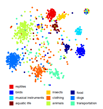 Frome et al., 2013
Please consider that while you may say "Obviously, a goldfish has to do more with a shark than with an iguana because they are both aquatic" you are comparing these across one dimension, namely natural habitat, while if you compared them by size the results would be different. These infinite dimensions across which you can compare two words are resumed into a finite number of categories which is what we call embeddings. In this image, we are arbitrarily choosing one dimension to make the point since it is intuitive to us human beings.
To create this network the authors combined a computer vision architecture with the embeddings data to create a hybrid model that we can see in the following picture:
 Frome et al., 2013
PATH = Path('../data/imagenet')
TMP_PATH = Path('../data/imagenet/tmp')
TRANS_PATH = Path('../data/translate/')
PATH_TRN = PATH/'train'
First we are going to load our word vectors. We'll see that each word has a normalized number between [-1, 1] for each of the 300 embeddings. This is effectively a 300 dimension representation of the meaning of each word. As an example, let's see the embedding for 'king'.
ft_vecs = ft.load_model(str((TRANS_PATH/'wiki.en.bin')))
ft_vecs.get_word_vector('king')
We can also see how correlated two words are in how close these numbers are for each embedding. For example we would stipulate that 'jeremy' and 'Jeremy' are more related than 'banana' and 'Jeremy'. Let's see if our embeddings think alike.
np.corrcoef(ft_vecs.get_word_vector('jeremy'), ft_vecs.get_word_vector('Jeremy'))
np.corrcoef(ft_vecs.get_word_vector('banana'), ft_vecs.get_word_vector('Jeremy'))
Map imagenet classes to word vectors
Next, we will get all the words in the dictionary and sort them by their frequency (how often do they appear in the aforementioned datasets). We will then count how many words do we have in our dictionary as another step in the 'discovery phase' of our data.
ft_words = ft_vecs.get_words(include_freq=True)
ft_word_dict = {k:v for k,v in zip(*ft_words)}
ft_words = sorted(ft_word_dict.keys(), key=lambda x: ft_word_dict[x])
We will download the names of our 1000 imagenet classes so that we can assign each class in our imagenet dataset to a 300-long embedding (for that we need the actual word-id for each class).
CLASSES_FN = 'imagenet_class_index.json'
download_url(f'http://files.fast.ai/models/{CLASSES_FN}', TMP_PATH/CLASSES_FN)
We will also download all the nouns in English from WORDNET.
WORDS_FN = 'classids.txt'
download_url(f'http://files.fast.ai/data/{WORDS_FN}', PATH/WORDS_FN)
Next we will build a dictionary that maps our classes to the word-id for each class.
class_dict = json.load((TMP_PATH/CLASSES_FN).open())
classids_1k = dict(class_dict.values())
nclass = len(class_dict); nclass
Now let's check that our class-id assignments are made correctly. Here we can see our two worlds:
- Imagenet and its class to id mapping
- WORDNET and its class to id mapping
class_dict['0']
classid_lines = (PATH/WORDS_FN).open().readlines()
classid_lines[:5]
Now we have the nouns in the English language and the Imagenet class ids, we need to connect each of these with the words in fastText. We will do this by creating a dictionary of synset to word vectors for both our WORDNET and Imagenet lists that will only keep the words that are present in both datasets (i.e. both WORDNET and fastText for syn_wv and both Imagenet and fastText for syn_wv_1k).
classids = dict(l.strip().split() for l in classid_lines)
len(classids),len(classids_1k)
lc_vec_d = {w.lower(): ft_vecs.get_word_vector(w) for w in ft_words[-1000000:]}
syn_wv = [(k, lc_vec_d[v.lower()]) for k,v in classids.items()
          if v.lower() in lc_vec_d]
syn_wv_1k = [(k, lc_vec_d[v.lower()]) for k,v in classids_1k.items()
          if v.lower() in lc_vec_d]
syn2wv = dict(syn_wv)
len(syn2wv), len(syn_wv_1k)
pickle.dump(syn2wv, (TMP_PATH/'syn2wv.pkl').open('wb'))
pickle.dump(syn_wv_1k, (TMP_PATH/'syn_wv_1k.pkl').open('wb'))
syn2wv = pickle.load((TMP_PATH/'syn2wv.pkl').open('rb'))
syn_wv_1k = pickle.load((TMP_PATH/'syn_wv_1k.pkl').open('rb'))
The next step is building the data we are going to train our model on. For that we are only including images with ids that are English nouns. Our x variables will be our images (which we are saving in a PosixPath format) and our y variables will be our vectors (300 floats, one for each embedding).
images = []
img_vecs = []
images_val = []
img_vecs_val = []

for d in (PATH/'train').iterdir():
    if d.name not in syn2wv: continue
    vec = syn2wv[d.name]
    for f in d.iterdir():
        images.append(str(f.relative_to(PATH)))
        img_vecs.append(vec)

n_val=0
for d in (PATH/'valid').iterdir():
    if d.name not in syn2wv: continue
    vec = syn2wv[d.name]
    for f in d.iterdir():
        images_val.append(str(f.relative_to(PATH)))
        img_vecs_val.append(vec)
        n_val += 1
n_val
img_vecs = np.stack(img_vecs)
img_vecs.shape
pickle.dump(images, (TMP_PATH/'images.pkl').open('wb'))
pickle.dump(img_vecs, (TMP_PATH/'img_vecs.pkl').open('wb'))
pickle.dump(images_val, (TMP_PATH/'images_val.pkl').open('wb'))
pickle.dump(img_vecs_val, (TMP_PATH/'img_vecs)val.pkl').open('wb'))
images = pickle.load((TMP_PATH/'images.pkl').open('rb'))
img_vecs = pickle.load((TMP_PATH/'img_vecs.pkl').open('rb'))
images_val = pickle.load((TMP_PATH/'images_val.pkl').open('rb'))
img_vecs_val = pickle.load((TMP_PATH/'img_vecs_val.pkl').open('rb'))
Getting the data ready
Let's build our dataset and create our DataBunch object. Note that we will need to tell our model how many classes we have. We will specify this manually since our ImageDataset class does not support it natively (this argument will then be passed to our model). We will resize our pictures to a 224x224 size and normalize them. Finally we will check that our data looks as we would like it to be.
folder_path = (PATH/"").absolute()
images = [folder_path/image for image in images]
images_val = [folder_path/image_val for image_val in images_val]
n = len(images); n
n_val = len(images_val); n_val
n+n_val
train_ds = ImageDataset(images, img_vecs)
valid_ds = ImageDataset(images_val, img_vecs_val)
train_ds.classes = range(300)
valid_ds.classes = range(300)
tfms = [[flip_lr(), crop_pad(size=224)], [flip_lr(), crop_pad(size=224)]]
data = DataBunch.create(train_ds, valid_ds, path=PATH, device=torch.device('cuda'), ds_tfms = tfms, tfms=imagenet_norm, size=224)
??get_transforms
len(data.train_dl)
x,y = next(iter(data.train_dl))
x.shape, y.shape
x[0],y[0]
len(data.valid_dl)
x_val,y_val = next(iter(data.valid_dl))
x_val.shape, y_val.shape
x_val[0],y_val[0]
from PIL import Image
Image.open(x)
Now it is time to train our model. Our model will try to predict the value of each embedding for each of our images. To accomplish this we will add a fully connected layer at the end of our resnet50 architecture (with 300 output neurons) and precompute the activations of the backbone model so as to save training time. We will also initialize the weights of the backbone model with the weights of the pretrained model. Given that the pretrained model and ours are both training in the same dataset we will not need to do any finetuning.
First we are going to start by precomputing our activations for the convolutional backbone and we will then train our head from these activations (so our model will not have to calculate them again for each epoch). Since we already have a pretrained backbone, we will just need to run one forward pass to compute the final activations; that is we will not need any optimization.
import bcolz, threading
from tqdm import tqdm
from torch.utils.data import Dataset
??ConvLearner
learn = ConvLearner(data, tvm.resnet50, ps=[0.2,0.2], lin_ftrs=[1024], pretrained=True, callback_fns=BnFreeze)
body = learn.model[0]
layers = list(body.children())
layers += [AdaptiveConcatPool2d(), Flatten()]
body = nn.Sequential(*layers)
body
nf = num_features(body)*2
nf
class FCDataset(Dataset):
    def __init__(self, x, y):
        self.x = x
        self.y = y

    def __getitem__(self, index):
        return (self.x[index], self.y[index])

    def __len__(self):
        return len(self.x)
learn.opt_fn = partial(AdamW, betas=(0.9,0.99))
def cos_loss(inp,targ): return 1 - F.cosine_similarity(inp,targ).mean()
learn.loss_fn = cos_loss
def get_activations(path, model_name, tmp_path, nf, force=False):
    tmpl = f'_{model_name}.bc'
    names = [os.path.join(path/'tmp', p+tmpl) for p in ('x_act', 'x_act_val')]
    if os.path.exists(names[0]) and not force:
        activations = [bcolz.open(p) for p in names]
    else:
        activations = [create_empty_bcolz(nf,p) for p in names]
    return activations
def create_empty_bcolz(n, name):
    return bcolz.carray(np.zeros((0,n), np.float32), chunklen=1, mode='w', rootdir=name)
def predict_to_bcolz(m, gen, arr, workers=4):
    arr.trim(len(arr))
    lock=threading.Lock()
    m.eval()
    for x,*_ in tqdm(gen):
        y = to_np(m(x.data).detach())
        with lock:
            arr.append(y)
    arr.flush()
def save_fc1(data, model, path, model_name, tmp_path, nf):
    act, val_act = get_activations(path, model_name, tmp_path, nf)
    m=model
    if len(act)!=len(data.train_ds):
        predict_to_bcolz(m, data.train_dl, act)
    if len(val_act)!=len(data.valid_ds):
        predict_to_bcolz(m, data.valid_dl, val_act)

    fc_data = FCDataset(act, img_vecs)
    fc_data_val = FCDataset(val_act, img_vecs_val)

    fc_data.classes = data.classes
    fc_data_val.classes = data.classes

    fc_db = DataBunch.create(fc_data, fc_data_val, path=PATH, device=torch.device('cuda'), bs=128)
    return fc_db
def num_features(m:Model)->int:
    "Return the number of output features for a `model`."
    for l in reversed(flatten_model(m)):
        if hasattr(l, 'num_features'):
            return l.num_features
fc_db = save_fc1(data, body, learn.path, 'resnet50', TMP_PATH, nf)
for x,y in iter(fc_db.valid_dl):
        print(x.shape, y.shape)
Now we are going to train our custom head from our computed activations. Notice that we are training our head as part of the original custom ConvNet and not as a separate sequential object. This is important because it means that we can load our pretrained model into our backbone like we did before, train our head only with the precomputed activations and then train the whole network without having to join our two parts (they are trained separately but are still connected in our memory). In summary, once we have loaded our pretrained weights on our backbone and trained our head we can directly train our whole network with differential learning rates without having to do any adjustment. Cool huh?
head = learn.model[1][2:]
head
learn_head = Learner(data=fc_db, model=head, opt_fn = partial(AdamW, betas=(0.9,0.99)), loss_fn = cos_loss)
learn_head.lr_find(start_lr=1e-4, end_lr=1e15)
learn_head.recorder.plot()
lr = 1e-3
wd = 1e-7
lr
learn_head.fit_one_cycle(cyc_len=2, max_lr=lr, wd=wd, div_factor=20, pct_start=0.2)
learn_head.save('pre0')
lrs = np.array([lr/1000,lr/100,lr])
learn.fit_one_cycle(3, lrs, wd=wd)
Image search
Search imagenet classes
syns, wvs = list(zip(*syn_wv_1k))
wvs = np.array(wvs)
%time pred_wv = learn.predict()
start=300
denorm = md.val_ds.denorm

def show_img(im, figsize=None, ax=None):
    if not ax: fig,ax = plt.subplots(figsize=figsize)
    ax.imshow(im)
    ax.axis('off')
    return ax

def show_imgs(ims, cols, figsize=None):
    fig,axes = plt.subplots(len(ims)//cols, cols, figsize=figsize)
    for i,ax in enumerate(axes.flat): show_img(ims[i], ax=ax)
    plt.tight_layout()
show_imgs(denorm(md.val_ds[start:start+25][0]), 5, (10,10))
import nmslib

def create_index(a):
    index = nmslib.init(space='angulardist')
    index.addDataPointBatch(a)
    index.createIndex()
    return index

def get_knns(index, vecs):
     return zip(*index.knnQueryBatch(vecs, k=10, num_threads=4))

def get_knn(index, vec): return index.knnQuery(vec, k=10)
nn_wvs = create_index(wvs)
idxs,dists = get_knns(nn_wvs, pred_wv)
[[classids[syns[id]] for id in ids[:3]] for ids in idxs[start:start+10]]
Search all wordnet noun classes
all_syns, all_wvs = list(zip(*syn2wv.items()))
all_wvs = np.array(all_wvs)
nn_allwvs = create_index(all_wvs)
idxs,dists = get_knns(nn_allwvs, pred_wv)
[[classids[all_syns[id]] for id in ids[:3]] for ids in idxs[start:start+10]]
Text -> image search
nn_predwv = create_index(pred_wv)
en_vecd = pickle.load(open(TRANS_PATH/'wiki.en.pkl','rb'))
vec = en_vecd['boat']
idxs,dists = get_knn(nn_predwv, vec)
show_imgs([open_image(PATH/md.val_ds.fnames[i]) for i in idxs[:3]], 3, figsize=(9,3));
vec = (en_vecd['engine'] + en_vecd['boat'])/2
idxs,dists = get_knn(nn_predwv, vec)
show_imgs([open_image(PATH/md.val_ds.fnames[i]) for i in idxs[:3]], 3, figsize=(9,3));
vec = (en_vecd['sail'] + en_vecd['boat'])/2
idxs,dists = get_knn(nn_predwv, vec)
show_imgs([open_image(PATH/md.val_ds.fnames[i]) for i in idxs[:3]], 3, figsize=(9,3));
Image->image
fname = 'valid/n01440764/ILSVRC2012_val_00007197.JPEG'
img = open_image(PATH/fname)
show_img(img);
t_img = md.val_ds.transform(img)
pred = learn.predict_array(t_img[None])
idxs,dists = get_knn(nn_predwv, pred)
show_imgs([open_image(PATH/md.val_ds.fnames[i]) for i in idxs[1:4]], 3, figsize=(9,3));