#!/usr/bin/env python
# coding: utf-8
# # Sentiment Classification the old-fashioned way:
# ## `Naive Bayes`, `Logistic Regression`, and `Ngrams`
# The purpose of this notebook is to show how sentiment classification is done via the classic techniques of `Naive Bayes`, `Logistic regression`, and `Ngrams`. We will be using `sklearn` and the `fastai` library.
#
# In a future lesson, we will revisit sentiment classification using `deep learning`, so that you can compare the two approaches.
# The content here was extended from [Lesson 10 of the fast.ai Machine Learning course](https://course.fast.ai/lessonsml1/lesson10.html). Linear model is pretty close to the state of the art here. Jeremy surpassed state of the art using a RNN in fall 2017.
# ## 0.The fastai library
# We will begin using [the fastai library](https://docs.fast.ai) (version 1.0) in this notebook. We will use it more once we move on to neural networks.
#
# The fastai library is built on top of PyTorch and encodes many state-of-the-art best practices. It is used in production at a number of companies. You can read more about it here:
#
# - [Fast.ai's software could radically democratize AI](https://www.zdnet.com/article/fast-ais-new-software-could-radically-democratize-ai/) (ZDNet)
#
# - [fastai v1 for PyTorch: Fast and accurate neural nets using modern best practices](https://www.fast.ai/2018/10/02/fastai-ai/) (fast.ai)
#
# - [fastai docs](https://docs.fast.ai/)
#
# ### Installation
#
# With conda:
#
# `conda install -c pytorch -c fastai fastai=1.0`
#
# Or with pip:
#
# `pip install fastai==1.0`
#
# More [installation information here](https://github.com/fastai/fastai/blob/master/README.md).
#
# Beginning in lesson 4, we will be using GPUs, so if you want, you could switch to a [cloud option](https://course.fast.ai/#using-a-gpu) now to setup fastai.
# ## 1. The IMDB dataset
#  # The [large movie review dataset](http://ai.stanford.edu/~amaas/data/sentiment/) contains a collection of 50,000 reviews from IMDB, We will use the version hosted as part [fast.ai datasets](https://course.fast.ai/datasets.html) on AWS Open Datasets.
#
# The dataset contains an even number of positive and negative reviews. The authors considered only highly polarized reviews. A negative review has a score ≤ 4 out of 10, and a positive review has a score ≥ 7 out of 10. Neutral reviews are not included in the dataset. The dataset is divided into training and test sets. The training set is the same 25,000 labeled reviews.
#
# The **sentiment classification task** consists of predicting the polarity (positive or negative) of a given text.
# ### Imports
# In[1]:
get_ipython().run_line_magic('reload_ext', 'autoreload')
get_ipython().run_line_magic('autoreload', '2')
get_ipython().run_line_magic('matplotlib', 'inline')
# In[2]:
from fastai import *
from fastai.text import *
from fastai.utils.mem import GPUMemTrace #call with mtrace
# In[3]:
import sklearn.feature_extraction.text as sklearn_text
import pickle
# ### Preview the sample IMDb data set
# fast.ai has a number of [datasets hosted via AWS Open Datasets](https://course.fast.ai/datasets.html) for easy download. We can see them by checking the docs for URLs (remember `??` is a helpful command):
# In[4]:
get_ipython().run_line_magic('pinfo2', ' URLs')
# It is always good to start working on a sample of your data before you use the full dataset-- this allows for quicker computations as you debug and get your code working. For IMDB, there is a sample dataset already available:
# In[5]:
path = untar_data(URLs.IMDB_SAMPLE)
path
# #### Read the data set into a pandas dataframe, which we can inspect to get a sense of what our data looks like. We see that the three columns contain review label, review text, and the `is_valid` flag, respectively. `is_valid` is a boolean flag indicating whether the row is from the validation set or not.
# In[6]:
df = pd.read_csv(path/'texts.csv')
df.head()
# ### Extract the movie reviews from the sample IMDb data set.
# #### We will be using [TextList](https://docs.fast.ai/text.data.html#TextList) from the fastai library:
# In[7]:
get_ipython().run_cell_magic('time', '', "# throws `BrokenProcessPool' Error sometimes. Keep trying `till it works!\n\ncount = 0\nerror = True\nwhile error:\n try: \n # Preprocessing steps\n movie_reviews = (TextList.from_csv(path, 'texts.csv', cols='text')\n .split_from_df(col=2)\n .label_from_df(cols=0))\n error = False\n print(f'failure count is {count}\\n') \n except: # catch *all* exceptions\n # accumulate failure count\n count = count + 1\n print(f'failure count is {count}')\n")
# ### Exploring IMDb review data
# A good first step for any data problem is to explore the data and get a sense of what it looks like. In this case we are looking at movie reviews, which have been labeled as "positive" or "negative". The reviews have already been `tokenized`, i.e. split into `tokens`, basic units such as words, prefixes, punctuation, capitalization, and other features of the text.
# In[8]:
movie_reviews
# ### Let's examine the`movie_reviews` object:
# In[9]:
dir(movie_reviews)
# ### `movie_reviews` splits the data into training and validation sets, `.train` and `.valid`
# In[10]:
print(f'There are {len(movie_reviews.train.x)} and {len(movie_reviews.valid.x)} reviews in the training and validations sets, respectively.')
# ### Reviews are composed of lists of tokens. In NLP, a **token** is the basic unit of processing (what the tokens are depends on the application and your choices). Here, the tokens mostly correspond to words or punctuation, as well as several special tokens, corresponding to unknown words, capitalization, etc.
# ### Special tokens:
# All those tokens starting with "xx" are fastai special tokens. You can see the list of all of them and their meanings ([in the fastai docs](https://docs.fast.ai/text.transform.html)):
#
# 
# ### Let's examine the structure of the `training set`
# #### movie_reviews.train is a `LabelList` object.
# #### movie_reviews.train.x is a `TextList` object that holds the reviews
# #### movie_reviews.train.y is a `CategoryList` object that holds the labels
# In[11]:
print(f'\fThere are {len(movie_reviews.train.x)} movie reviews in the training set\n')
print(movie_reviews.train)
# #### The text of the movie review is stored as a character `string`, which contains the tokens separated by spaces. Here is the text of the first review:
# In[12]:
print(movie_reviews.train.x[0].text)
print(f'\nThere are {len(movie_reviews.train.x[0].text)} characters in the review')
# #### The text string can be split to get the list of tokens.
# In[13]:
print(movie_reviews.train.x[0].text.split())
print(f'\nThe review has {len(movie_reviews.train.x[0].text.split())} tokens')
# #### The review tokens are `numericalized`, ie. mapped to integers. So a movie review is also stored as an array of integers:
# In[14]:
print(movie_reviews.train.x[0].data)
print(f'\nThe array contains {len(movie_reviews.train.x[0].data)} numericalized tokens')
# ## 2. The IMDb Vocabulary
# ### The `movie_revews` object also contains a `.vocab` property, even though it is not shown with`dir()`. (This may be an error in the `fastai` library.)
# In[15]:
movie_reviews.vocab
# ### The `vocab` object is a kind of reversible dictionary that translates back and forth between tokens and their integer representations. It has two methods of particular interest: `stoi` and `itos`, which stand for `string-to-index` and `index-to-string`
# #### `movie_reviews.vocab.stoi` maps vocabulary tokens to their `indexes` in vocab
# In[16]:
movie_reviews.vocab.stoi
# #### `movie_reviews.vocab.itos` maps the `indexes` of vocabulary tokens to `strings`
# In[17]:
movie_reviews.vocab.itos
# #### Notice that ints-to-string and string-to-ints have different lengths. Think for a moment about why this is.
# See Hint below
# In[18]:
print('itos ', 'length ',len(movie_reviews.vocab.itos),type(movie_reviews.vocab.itos) )
print('stoi ', 'length ',len(movie_reviews.vocab.stoi),type(movie_reviews.vocab.stoi) )
# #### Hint: `stoi` is an instance of the class `defaultdict`
#
# The [large movie review dataset](http://ai.stanford.edu/~amaas/data/sentiment/) contains a collection of 50,000 reviews from IMDB, We will use the version hosted as part [fast.ai datasets](https://course.fast.ai/datasets.html) on AWS Open Datasets.
#
# The dataset contains an even number of positive and negative reviews. The authors considered only highly polarized reviews. A negative review has a score ≤ 4 out of 10, and a positive review has a score ≥ 7 out of 10. Neutral reviews are not included in the dataset. The dataset is divided into training and test sets. The training set is the same 25,000 labeled reviews.
#
# The **sentiment classification task** consists of predicting the polarity (positive or negative) of a given text.
# ### Imports
# In[1]:
get_ipython().run_line_magic('reload_ext', 'autoreload')
get_ipython().run_line_magic('autoreload', '2')
get_ipython().run_line_magic('matplotlib', 'inline')
# In[2]:
from fastai import *
from fastai.text import *
from fastai.utils.mem import GPUMemTrace #call with mtrace
# In[3]:
import sklearn.feature_extraction.text as sklearn_text
import pickle
# ### Preview the sample IMDb data set
# fast.ai has a number of [datasets hosted via AWS Open Datasets](https://course.fast.ai/datasets.html) for easy download. We can see them by checking the docs for URLs (remember `??` is a helpful command):
# In[4]:
get_ipython().run_line_magic('pinfo2', ' URLs')
# It is always good to start working on a sample of your data before you use the full dataset-- this allows for quicker computations as you debug and get your code working. For IMDB, there is a sample dataset already available:
# In[5]:
path = untar_data(URLs.IMDB_SAMPLE)
path
# #### Read the data set into a pandas dataframe, which we can inspect to get a sense of what our data looks like. We see that the three columns contain review label, review text, and the `is_valid` flag, respectively. `is_valid` is a boolean flag indicating whether the row is from the validation set or not.
# In[6]:
df = pd.read_csv(path/'texts.csv')
df.head()
# ### Extract the movie reviews from the sample IMDb data set.
# #### We will be using [TextList](https://docs.fast.ai/text.data.html#TextList) from the fastai library:
# In[7]:
get_ipython().run_cell_magic('time', '', "# throws `BrokenProcessPool' Error sometimes. Keep trying `till it works!\n\ncount = 0\nerror = True\nwhile error:\n try: \n # Preprocessing steps\n movie_reviews = (TextList.from_csv(path, 'texts.csv', cols='text')\n .split_from_df(col=2)\n .label_from_df(cols=0))\n error = False\n print(f'failure count is {count}\\n') \n except: # catch *all* exceptions\n # accumulate failure count\n count = count + 1\n print(f'failure count is {count}')\n")
# ### Exploring IMDb review data
# A good first step for any data problem is to explore the data and get a sense of what it looks like. In this case we are looking at movie reviews, which have been labeled as "positive" or "negative". The reviews have already been `tokenized`, i.e. split into `tokens`, basic units such as words, prefixes, punctuation, capitalization, and other features of the text.
# In[8]:
movie_reviews
# ### Let's examine the`movie_reviews` object:
# In[9]:
dir(movie_reviews)
# ### `movie_reviews` splits the data into training and validation sets, `.train` and `.valid`
# In[10]:
print(f'There are {len(movie_reviews.train.x)} and {len(movie_reviews.valid.x)} reviews in the training and validations sets, respectively.')
# ### Reviews are composed of lists of tokens. In NLP, a **token** is the basic unit of processing (what the tokens are depends on the application and your choices). Here, the tokens mostly correspond to words or punctuation, as well as several special tokens, corresponding to unknown words, capitalization, etc.
# ### Special tokens:
# All those tokens starting with "xx" are fastai special tokens. You can see the list of all of them and their meanings ([in the fastai docs](https://docs.fast.ai/text.transform.html)):
#
# 
# ### Let's examine the structure of the `training set`
# #### movie_reviews.train is a `LabelList` object.
# #### movie_reviews.train.x is a `TextList` object that holds the reviews
# #### movie_reviews.train.y is a `CategoryList` object that holds the labels
# In[11]:
print(f'\fThere are {len(movie_reviews.train.x)} movie reviews in the training set\n')
print(movie_reviews.train)
# #### The text of the movie review is stored as a character `string`, which contains the tokens separated by spaces. Here is the text of the first review:
# In[12]:
print(movie_reviews.train.x[0].text)
print(f'\nThere are {len(movie_reviews.train.x[0].text)} characters in the review')
# #### The text string can be split to get the list of tokens.
# In[13]:
print(movie_reviews.train.x[0].text.split())
print(f'\nThe review has {len(movie_reviews.train.x[0].text.split())} tokens')
# #### The review tokens are `numericalized`, ie. mapped to integers. So a movie review is also stored as an array of integers:
# In[14]:
print(movie_reviews.train.x[0].data)
print(f'\nThe array contains {len(movie_reviews.train.x[0].data)} numericalized tokens')
# ## 2. The IMDb Vocabulary
# ### The `movie_revews` object also contains a `.vocab` property, even though it is not shown with`dir()`. (This may be an error in the `fastai` library.)
# In[15]:
movie_reviews.vocab
# ### The `vocab` object is a kind of reversible dictionary that translates back and forth between tokens and their integer representations. It has two methods of particular interest: `stoi` and `itos`, which stand for `string-to-index` and `index-to-string`
# #### `movie_reviews.vocab.stoi` maps vocabulary tokens to their `indexes` in vocab
# In[16]:
movie_reviews.vocab.stoi
# #### `movie_reviews.vocab.itos` maps the `indexes` of vocabulary tokens to `strings`
# In[17]:
movie_reviews.vocab.itos
# #### Notice that ints-to-string and string-to-ints have different lengths. Think for a moment about why this is.
# See Hint below
# In[18]:
print('itos ', 'length ',len(movie_reviews.vocab.itos),type(movie_reviews.vocab.itos) )
print('stoi ', 'length ',len(movie_reviews.vocab.stoi),type(movie_reviews.vocab.stoi) )
# #### Hint: `stoi` is an instance of the class `defaultdict`
#  # #### In a `defaultdict`, rare words that appear fewer than three times in the corpus, and words that are not in the dictionary, are mapped to a `default value`, in this case, zero
# In[19]:
rare_words = ['acrid','a_random_made_up_nonexistant_word','acrimonious','allosteric','anodyne','antikythera']
for word in rare_words:
print(movie_reviews.vocab.stoi[word])
# #### What's the `token` corresponding to the `default` value?
# In[20]:
print(movie_reviews.vocab.itos[0])
# #### Note that `stoi` (string-to-int) is larger than `itos` (int-to-string).
# In[21]:
print(f'len(stoi) = {len(movie_reviews.vocab.stoi)}')
print(f'len(itos) = {len(movie_reviews.vocab.itos)}')
print(f'len(stoi) - len(itos) = {len(movie_reviews.vocab.stoi) - len(movie_reviews.vocab.itos)}')
# #### This is because many words map to `unknown`. We can confirm here:
# In[22]:
unk = []
for word, num in movie_reviews.vocab.stoi.items():
if num==0:
unk.append(word)
# In[23]:
len(unk)
# #### Question: why isn't len(unk) = len(stoi) - len(itos)?
# Hint: remember the list of rare words we used to query `stoi` a few cells back?
# #### Here are the first 25 words that are mapped to `unknown`
# In[24]:
unk[:25]
# ## 3. Map the movie reviews into a vector space
# ### There are 6016 unique tokens in the IMDb review vocabulary. Their numericalized values range from 0 to 6015
# In[25]:
print(f'There are {len(movie_reviews.vocab.itos)} unique tokens in the IMDb review sample vocabulary')
print(f'The numericalized token values run from {min(movie_reviews.vocab.stoi.values())} to {max(movie_reviews.vocab.stoi.values())} ')
# ### Each review can be mapped to a 6016-dimensional `embedding vector` whose indices correspond to the numericalized tokens, and whose values are the number of times the corresponding token appeared in the review. To do this efficiently we need to learn a bit about `Counters`.
# ### 3A. Counters
# A **Counter** is a useful Python object. A **Counter** applied to a list returns an ordered dictionary whose keys are the unique elements in the list, and whose values are the counts of the unique elements. Counters are from the collections module (along with OrderedDict, defaultdict, deque, and namedtuple).
# Here is how Counters work:
# #### Let's make a TokenCounter for movie reviews
# In[26]:
TokenCounter = lambda review_index : Counter((movie_reviews.train.x)[review_index].data)
TokenCounter(0).items()
# #### The TokenCounter `keys` are the numericalized `tokens` that apper in the review
# In[27]:
TokenCounter(0).keys()
# #### The TokenCounter `values` are the `token multiplicities`, i.e the number of times each `token` appears in the review
# In[28]:
TokenCounter(0).values()
# ### 3B. Mapping movie reviews to `embedding vectors`
# #### Make a `count_vectorizer` function that represents a movie review as a 6016-dimensional `embedding vector`
# #### The `indices` of the `embedding vector` correspond to the n6016 numericalized tokens in the vocabulary; the `values` specify how often the corresponding token appears in the review.
# In[29]:
n_terms = len(movie_reviews.vocab.itos)
n_docs = len(movie_reviews.train.x)
make_token_counter = lambda review_index: Counter(movie_reviews.train.x[review_index].data)
def count_vectorizer(review_index,n_terms = n_terms,make_token_counter = make_token_counter):
# input: review index, n_terms, and tokenizer function
# output: embedding vector for the review
embedding_vector = np.zeros(n_terms)
keys = list(make_token_counter(review_index).keys())
values = list(make_token_counter(review_index).values())
embedding_vector[keys] = values
return embedding_vector
# make the embedding vector for the first review
embedding_vector = count_vectorizer(0)
# #### Here is the `embedding vector` for the first review in the training data set
# In[30]:
print(f'The review is embedded in a {len(embedding_vector)} dimensional vector')
embedding_vector
# ## 4. Create the document-term matrix for the IMDb
# #### In non-deep learning methods of NLP, we are often interested only in `which words` were used in a review, and `how often each word got used`. This is known as the `bag of words` approach, and it suggests a really simple way to store a document (in this case, a movie review).
#
# #### For each review we can keep track of which words were used and how often each word was used with a `vector` whose `length` is the number of tokens in the vocabulary, which we will call `n`. The `indexes` of this `vector` correspond to the `tokens` in the `IMDb vocabulary`, and the`values` of the vector are the number of times the corresponding tokens appeared in the review. For example the values stored at indexes 0, 1, 2, 3, 4 of the vector record the number of times the 5 tokens ['xxunk','xxpad','xxbos','xxeos','xxfld'] appeared in the review, respectively.
#
# #### Now, if our movie review database has `m` reviews, and each review is represented by a `vector` of length `n`, then vertically stacking the row vectors for all the reviews creates a matrix representation of the IMDb, which we call its `document-term matrix`. The `rows` correspond to `documents` (reviews), while the `columns` correspond to `terms` (or tokens in the vocabulary).
# In the previous lesson, we used [sklearn's CountVectorizer](https://github.com/scikit-learn/scikit-learn/blob/55bf5d9/sklearn/feature_extraction/text.py#L940) to generate the `vectors` that represent individual reviews. Today we will create our own (similar) version. This is for two reasons:
# - to understand what sklearn is doing underneath the hood
# - to create something that will work with a fastai TextList
# ### Form the embedding vectors for the movie_reviews in the training set and stack them vertically
# In[31]:
# Define a function to build the full document-term matrix
print(f'there are {n_docs} reviews, and {n_terms} unique tokens in the vocabulary')
def make_full_doc_term_matrix(count_vectorizer,n_terms=n_terms,n_docs=n_docs):
# loop through the movie reviews
for doc_index in range(n_docs):
# make the embedding vector for the current review
embedding_vector = count_vectorizer(doc_index,n_terms)
# append the embedding vector to the document-term matrix
if(doc_index == 0):
A = embedding_vector
else:
A = np.vstack((A,embedding_vector))
# return the document-term matrix
return A
# Build the full document term matrix for the movie_reviews training set
A = make_full_doc_term_matrix(count_vectorizer)
# ### Explore the `sparsity` of the document-term matrix
# #### The `sparsity` of a matrix is defined as the fraction of of zero-valued elements
# In[32]:
NNZ = np.count_nonzero(A)
sparsity = (A.size-NNZ)/A.size
print(f'Only {NNZ} of the {A.size} elements in the document-term matrix are nonzero')
print(f'The sparsity of the document-term matrix is {sparsity}')
# #### Using matplotlib's `spy` method, we can visualize the structure of the `document-term matrix`
# `spy` plots the array, indicating each non-zero value with a dot.
# In[33]:
fig = plt.figure()
plt.spy(A, markersize=0.10, aspect = 'auto')
fig.set_size_inches(8,6)
fig.savefig('doc_term_matrix.png', dpi=800)
# #### Several observations stand out:
# 1. Evidently, the document-term matrix is `sparse` ie. has a high proportion of zeros!
# 2. The density of the matrix increases toward the `left` edge. This makes sense because the tokens are ordered by usage frequency, with frequency increasing toward the `left`.
# 3. There is a perplexing pattern of curved vertical `density ripples`. If anyone has an explanation, please let me know!
#
# #### Next we'll see how to exploit matrix sparsity to save memory storage space, and compute time and resources.
#
# ## 5. Sparse Matrix Representation
# #### Even though we've reduced over 19,000 unique words in our corpus of reviews down to a vocabulary of 6,000 words, that's still a lot! But reviews are generally short, a few hundred words. So most tokens don't appear in a typical review. That means that most of the entries in the document-term matrix will be zeros, and therefore ordinary matrix operations will waste a lot of compute resources multiplying and adding zeros.
#
# #### We want to maximize the use of space and time by storing and performing matrix operations on our document-term matrix as a **sparse matrix**. `scipy` provides tools for efficient sparse matrix representatin and operations.
# #### Loosely speaking, matrix with a high proportion of zeros is called `sparse` (the opposite of sparse is `dense`). For sparse matrices, you can save a lot of memory by only storing the non-zero values.
#
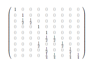
# #### More specifically, a class of matrices is called **sparse** if the number of non-zero elements is proportional to the number of rows (or columns) instead of being proportional to the product rows x columns. An example is the class of diagonal matrices.
#
#
#
# #### In a `defaultdict`, rare words that appear fewer than three times in the corpus, and words that are not in the dictionary, are mapped to a `default value`, in this case, zero
# In[19]:
rare_words = ['acrid','a_random_made_up_nonexistant_word','acrimonious','allosteric','anodyne','antikythera']
for word in rare_words:
print(movie_reviews.vocab.stoi[word])
# #### What's the `token` corresponding to the `default` value?
# In[20]:
print(movie_reviews.vocab.itos[0])
# #### Note that `stoi` (string-to-int) is larger than `itos` (int-to-string).
# In[21]:
print(f'len(stoi) = {len(movie_reviews.vocab.stoi)}')
print(f'len(itos) = {len(movie_reviews.vocab.itos)}')
print(f'len(stoi) - len(itos) = {len(movie_reviews.vocab.stoi) - len(movie_reviews.vocab.itos)}')
# #### This is because many words map to `unknown`. We can confirm here:
# In[22]:
unk = []
for word, num in movie_reviews.vocab.stoi.items():
if num==0:
unk.append(word)
# In[23]:
len(unk)
# #### Question: why isn't len(unk) = len(stoi) - len(itos)?
# Hint: remember the list of rare words we used to query `stoi` a few cells back?
# #### Here are the first 25 words that are mapped to `unknown`
# In[24]:
unk[:25]
# ## 3. Map the movie reviews into a vector space
# ### There are 6016 unique tokens in the IMDb review vocabulary. Their numericalized values range from 0 to 6015
# In[25]:
print(f'There are {len(movie_reviews.vocab.itos)} unique tokens in the IMDb review sample vocabulary')
print(f'The numericalized token values run from {min(movie_reviews.vocab.stoi.values())} to {max(movie_reviews.vocab.stoi.values())} ')
# ### Each review can be mapped to a 6016-dimensional `embedding vector` whose indices correspond to the numericalized tokens, and whose values are the number of times the corresponding token appeared in the review. To do this efficiently we need to learn a bit about `Counters`.
# ### 3A. Counters
# A **Counter** is a useful Python object. A **Counter** applied to a list returns an ordered dictionary whose keys are the unique elements in the list, and whose values are the counts of the unique elements. Counters are from the collections module (along with OrderedDict, defaultdict, deque, and namedtuple).
# Here is how Counters work:
# #### Let's make a TokenCounter for movie reviews
# In[26]:
TokenCounter = lambda review_index : Counter((movie_reviews.train.x)[review_index].data)
TokenCounter(0).items()
# #### The TokenCounter `keys` are the numericalized `tokens` that apper in the review
# In[27]:
TokenCounter(0).keys()
# #### The TokenCounter `values` are the `token multiplicities`, i.e the number of times each `token` appears in the review
# In[28]:
TokenCounter(0).values()
# ### 3B. Mapping movie reviews to `embedding vectors`
# #### Make a `count_vectorizer` function that represents a movie review as a 6016-dimensional `embedding vector`
# #### The `indices` of the `embedding vector` correspond to the n6016 numericalized tokens in the vocabulary; the `values` specify how often the corresponding token appears in the review.
# In[29]:
n_terms = len(movie_reviews.vocab.itos)
n_docs = len(movie_reviews.train.x)
make_token_counter = lambda review_index: Counter(movie_reviews.train.x[review_index].data)
def count_vectorizer(review_index,n_terms = n_terms,make_token_counter = make_token_counter):
# input: review index, n_terms, and tokenizer function
# output: embedding vector for the review
embedding_vector = np.zeros(n_terms)
keys = list(make_token_counter(review_index).keys())
values = list(make_token_counter(review_index).values())
embedding_vector[keys] = values
return embedding_vector
# make the embedding vector for the first review
embedding_vector = count_vectorizer(0)
# #### Here is the `embedding vector` for the first review in the training data set
# In[30]:
print(f'The review is embedded in a {len(embedding_vector)} dimensional vector')
embedding_vector
# ## 4. Create the document-term matrix for the IMDb
# #### In non-deep learning methods of NLP, we are often interested only in `which words` were used in a review, and `how often each word got used`. This is known as the `bag of words` approach, and it suggests a really simple way to store a document (in this case, a movie review).
#
# #### For each review we can keep track of which words were used and how often each word was used with a `vector` whose `length` is the number of tokens in the vocabulary, which we will call `n`. The `indexes` of this `vector` correspond to the `tokens` in the `IMDb vocabulary`, and the`values` of the vector are the number of times the corresponding tokens appeared in the review. For example the values stored at indexes 0, 1, 2, 3, 4 of the vector record the number of times the 5 tokens ['xxunk','xxpad','xxbos','xxeos','xxfld'] appeared in the review, respectively.
#
# #### Now, if our movie review database has `m` reviews, and each review is represented by a `vector` of length `n`, then vertically stacking the row vectors for all the reviews creates a matrix representation of the IMDb, which we call its `document-term matrix`. The `rows` correspond to `documents` (reviews), while the `columns` correspond to `terms` (or tokens in the vocabulary).
# In the previous lesson, we used [sklearn's CountVectorizer](https://github.com/scikit-learn/scikit-learn/blob/55bf5d9/sklearn/feature_extraction/text.py#L940) to generate the `vectors` that represent individual reviews. Today we will create our own (similar) version. This is for two reasons:
# - to understand what sklearn is doing underneath the hood
# - to create something that will work with a fastai TextList
# ### Form the embedding vectors for the movie_reviews in the training set and stack them vertically
# In[31]:
# Define a function to build the full document-term matrix
print(f'there are {n_docs} reviews, and {n_terms} unique tokens in the vocabulary')
def make_full_doc_term_matrix(count_vectorizer,n_terms=n_terms,n_docs=n_docs):
# loop through the movie reviews
for doc_index in range(n_docs):
# make the embedding vector for the current review
embedding_vector = count_vectorizer(doc_index,n_terms)
# append the embedding vector to the document-term matrix
if(doc_index == 0):
A = embedding_vector
else:
A = np.vstack((A,embedding_vector))
# return the document-term matrix
return A
# Build the full document term matrix for the movie_reviews training set
A = make_full_doc_term_matrix(count_vectorizer)
# ### Explore the `sparsity` of the document-term matrix
# #### The `sparsity` of a matrix is defined as the fraction of of zero-valued elements
# In[32]:
NNZ = np.count_nonzero(A)
sparsity = (A.size-NNZ)/A.size
print(f'Only {NNZ} of the {A.size} elements in the document-term matrix are nonzero')
print(f'The sparsity of the document-term matrix is {sparsity}')
# #### Using matplotlib's `spy` method, we can visualize the structure of the `document-term matrix`
# `spy` plots the array, indicating each non-zero value with a dot.
# In[33]:
fig = plt.figure()
plt.spy(A, markersize=0.10, aspect = 'auto')
fig.set_size_inches(8,6)
fig.savefig('doc_term_matrix.png', dpi=800)
# #### Several observations stand out:
# 1. Evidently, the document-term matrix is `sparse` ie. has a high proportion of zeros!
# 2. The density of the matrix increases toward the `left` edge. This makes sense because the tokens are ordered by usage frequency, with frequency increasing toward the `left`.
# 3. There is a perplexing pattern of curved vertical `density ripples`. If anyone has an explanation, please let me know!
#
# #### Next we'll see how to exploit matrix sparsity to save memory storage space, and compute time and resources.
#
# ## 5. Sparse Matrix Representation
# #### Even though we've reduced over 19,000 unique words in our corpus of reviews down to a vocabulary of 6,000 words, that's still a lot! But reviews are generally short, a few hundred words. So most tokens don't appear in a typical review. That means that most of the entries in the document-term matrix will be zeros, and therefore ordinary matrix operations will waste a lot of compute resources multiplying and adding zeros.
#
# #### We want to maximize the use of space and time by storing and performing matrix operations on our document-term matrix as a **sparse matrix**. `scipy` provides tools for efficient sparse matrix representatin and operations.
# #### Loosely speaking, matrix with a high proportion of zeros is called `sparse` (the opposite of sparse is `dense`). For sparse matrices, you can save a lot of memory by only storing the non-zero values.
#
# #### More specifically, a class of matrices is called **sparse** if the number of non-zero elements is proportional to the number of rows (or columns) instead of being proportional to the product rows x columns. An example is the class of diagonal matrices.
#
#
#  #
#
# ### Visualizing sparse matrix structure
#
#
#
# ### Visualizing sparse matrix structure
#  # ref. https://scipy-lectures.org/advanced/scipy_sparse/introduction.html
# ### Sparse matrix storage formats
#
#
# ref. https://scipy-lectures.org/advanced/scipy_sparse/introduction.html
# ### Sparse matrix storage formats
#
#  # ref. https://scipy-lectures.org/advanced/scipy_sparse/storage_schemes.html
#
# There are the most common sparse storage formats:
# - coordinate-wise (scipy calls COO)
# - compressed sparse row (CSR)
# - compressed sparse column (CSC)
#
#
# ### Definition of the Compressed Sparse Row (CSR) format
#
# Let's start out with a presecription for the **CSR format** (ref. https://en.wikipedia.org/wiki/Sparse_matrix)
#
# Given a full matrix **`A`** that has **`m`** rows, **`n`** columns, and **`N`** nonzero values, the CSR (Compressed Sparse Row) representation uses three arrays as follows:
#
# 1. **`Val[0:N]`** contains the **values** of the **`N` non-zero elements**.
#
# 2. **`Col[0:N]`** contains the **column indices** of the **`N` non-zero elements**.
#
# 3. For each row **`i`** of **`A`**, **`RowPointer[i]`** contains the index in **Val** of the the first **nonzero value** in row **`i`**. If there are no nonzero values in the **ith** row, then **`RowPointer[i] = None`**. And, by convention, an extra value **`RowPointer[m] = N`** is tacked on at the end.
#
# Question: How many floats and ints does it take to store the matrix **`A`** in CSR format?
#
# Let's walk through [a few examples](http://www.mathcs.emory.edu/~cheung/Courses/561/Syllabus/3-C/sparse.html) at the Emory University website
#
#
# ## 6. Store the document-term matrix in CSR format
# i.e. given the `TextList` object containing the list of reviews, return the three arrays (values, column_indices, row_pointer)
# ### Scipy Implementation of sparse matrices
#
# From the [Scipy Sparse Matrix Documentation](https://docs.scipy.org/doc/scipy-0.18.1/reference/sparse.html)
#
# - To construct a matrix efficiently, use either dok_matrix or lil_matrix. The lil_matrix class supports basic slicing and fancy indexing with a similar syntax to NumPy arrays. As illustrated below, the COO format may also be used to efficiently construct matrices
# - To perform manipulations such as multiplication or inversion, first convert the matrix to either CSC or CSR format.
# - All conversions among the CSR, CSC, and COO formats are efficient, linear-time operations.
# ### To really understand the CSR format, we need to be able know how to do two things:
# 1. Translate a regular matrix A into CSR format
# 2. Reconstruct a regular matrix from its CSR sparse representation
#
# ### 6.1. Translate a regular matrix A into CSR format
# This is done by implementing the definition of `CSR format`, given above.
# In[34]:
# construct the document-term matrix in CSR format
# i.e. return (values, column_indices, row_pointer)
def get_doc_term_matrix(text_list, n_terms):
# inputs:
# text_list, a TextList object
# n_terms, the number of tokens in our IMDb vocabulary
# output:
# the CSR format sparse representation of the document-term matrix in the form of a
# scipy.sparse.csr.csr_matrix object
# initialize arrays
values = []
column_indices = []
row_pointer = []
row_pointer.append(0)
# from the TextList object
for _, doc in enumerate(text_list):
feature_counter = Counter(doc.data)
column_indices.extend(feature_counter.keys())
values.extend(feature_counter.values())
# Tack on N (number of nonzero elements in the matrix) to the end of the row_pointer array
row_pointer.append(len(values))
return scipy.sparse.csr_matrix((values, column_indices, row_pointer),
shape=(len(row_pointer) - 1, n_terms),
dtype=int)
# #### Get the document-term matrix in CSR format for the training data
# In[35]:
get_ipython().run_cell_magic('time', '', 'train_doc_term = get_doc_term_matrix(movie_reviews.train.x, len(movie_reviews.vocab.itos))\n')
# In[36]:
type(train_doc_term)
# In[37]:
train_doc_term.shape
# #### Get the document-term matrix in CSR format for the validation data
# In[38]:
get_ipython().run_cell_magic('time', '', 'valid_doc_term = get_doc_term_matrix(movie_reviews.valid.x, len(movie_reviews.vocab.itos))\n')
# In[39]:
type(valid_doc_term)
# In[40]:
valid_doc_term.shape
# ### 6.2 Reconstruct a regular matrix from its CSR sparse representation
# #### Given a CSR format sparse matrix representation $(\text{values},\text{column_indices}, \text{row_pointer})$ of a $\text{m}\times \text{n}$ matrix $\text{A}$,
# ref. https://scipy-lectures.org/advanced/scipy_sparse/storage_schemes.html
#
# There are the most common sparse storage formats:
# - coordinate-wise (scipy calls COO)
# - compressed sparse row (CSR)
# - compressed sparse column (CSC)
#
#
# ### Definition of the Compressed Sparse Row (CSR) format
#
# Let's start out with a presecription for the **CSR format** (ref. https://en.wikipedia.org/wiki/Sparse_matrix)
#
# Given a full matrix **`A`** that has **`m`** rows, **`n`** columns, and **`N`** nonzero values, the CSR (Compressed Sparse Row) representation uses three arrays as follows:
#
# 1. **`Val[0:N]`** contains the **values** of the **`N` non-zero elements**.
#
# 2. **`Col[0:N]`** contains the **column indices** of the **`N` non-zero elements**.
#
# 3. For each row **`i`** of **`A`**, **`RowPointer[i]`** contains the index in **Val** of the the first **nonzero value** in row **`i`**. If there are no nonzero values in the **ith** row, then **`RowPointer[i] = None`**. And, by convention, an extra value **`RowPointer[m] = N`** is tacked on at the end.
#
# Question: How many floats and ints does it take to store the matrix **`A`** in CSR format?
#
# Let's walk through [a few examples](http://www.mathcs.emory.edu/~cheung/Courses/561/Syllabus/3-C/sparse.html) at the Emory University website
#
#
# ## 6. Store the document-term matrix in CSR format
# i.e. given the `TextList` object containing the list of reviews, return the three arrays (values, column_indices, row_pointer)
# ### Scipy Implementation of sparse matrices
#
# From the [Scipy Sparse Matrix Documentation](https://docs.scipy.org/doc/scipy-0.18.1/reference/sparse.html)
#
# - To construct a matrix efficiently, use either dok_matrix or lil_matrix. The lil_matrix class supports basic slicing and fancy indexing with a similar syntax to NumPy arrays. As illustrated below, the COO format may also be used to efficiently construct matrices
# - To perform manipulations such as multiplication or inversion, first convert the matrix to either CSC or CSR format.
# - All conversions among the CSR, CSC, and COO formats are efficient, linear-time operations.
# ### To really understand the CSR format, we need to be able know how to do two things:
# 1. Translate a regular matrix A into CSR format
# 2. Reconstruct a regular matrix from its CSR sparse representation
#
# ### 6.1. Translate a regular matrix A into CSR format
# This is done by implementing the definition of `CSR format`, given above.
# In[34]:
# construct the document-term matrix in CSR format
# i.e. return (values, column_indices, row_pointer)
def get_doc_term_matrix(text_list, n_terms):
# inputs:
# text_list, a TextList object
# n_terms, the number of tokens in our IMDb vocabulary
# output:
# the CSR format sparse representation of the document-term matrix in the form of a
# scipy.sparse.csr.csr_matrix object
# initialize arrays
values = []
column_indices = []
row_pointer = []
row_pointer.append(0)
# from the TextList object
for _, doc in enumerate(text_list):
feature_counter = Counter(doc.data)
column_indices.extend(feature_counter.keys())
values.extend(feature_counter.values())
# Tack on N (number of nonzero elements in the matrix) to the end of the row_pointer array
row_pointer.append(len(values))
return scipy.sparse.csr_matrix((values, column_indices, row_pointer),
shape=(len(row_pointer) - 1, n_terms),
dtype=int)
# #### Get the document-term matrix in CSR format for the training data
# In[35]:
get_ipython().run_cell_magic('time', '', 'train_doc_term = get_doc_term_matrix(movie_reviews.train.x, len(movie_reviews.vocab.itos))\n')
# In[36]:
type(train_doc_term)
# In[37]:
train_doc_term.shape
# #### Get the document-term matrix in CSR format for the validation data
# In[38]:
get_ipython().run_cell_magic('time', '', 'valid_doc_term = get_doc_term_matrix(movie_reviews.valid.x, len(movie_reviews.vocab.itos))\n')
# In[39]:
type(valid_doc_term)
# In[40]:
valid_doc_term.shape
# ### 6.2 Reconstruct a regular matrix from its CSR sparse representation
# #### Given a CSR format sparse matrix representation $(\text{values},\text{column_indices}, \text{row_pointer})$ of a $\text{m}\times \text{n}$ matrix $\text{A}$,
how can we recover $\text{A}$?
#
# First create $\text{m}\times \text{n}$ matrix with all zeros.
# We will recover $\text{A}$ by overwriting the entries in the zeros matrix row by row with the non-zero entries in $\text{A}$ as follows:
# In[41]:
def CSR_to_full(values, column_indices, row_ptr, m,n):
A = zeros(m,n)
for row in range(n):
if row_ptr is not null:
A[row,column_indices[row_ptr[row]:row_ptr[row+1]]] = values[row_ptr[row]:row_ptr[row+1]]
return A
# ## 7. IMDb data exploration exercises
# #### The`.todense()` method converts a sparse matrix back to a regular (dense) matrix.
# In[42]:
valid_doc_term
# In[43]:
valid_doc_term.todense()[:10,:10]
# #### Consider the second review in the validation set
# In[44]:
review = movie_reviews.valid.x[1]
review
# **Exercise 1:** How many times does the word "it" appear in this review? Confirm that the correct values is stored in the document-term matrix, for the row corresponding to this review and the column corresponding to the word "it".
# #### Answer 1:
# In[45]:
# try it!
# Your code here.
# **Exercise 2**: Confirm that the review has 144 tokens, 81 of which are distinct
# #### Answer 2:
# In[46]:
valid_doc_term[1]
# In[47]:
valid_doc_term[1].sum()
# In[48]:
len(set(review.data))
# **Exercise 3:** How could you convert review.data back to text (without just using review.text)?
# In[49]:
review.data
# #### Answer 3:
# In[50]:
word_list = [movie_reviews.vocab.itos[a] for a in review.data]
print(word_list)
# In[51]:
reconstructed_text = ' '.join(word_list)
print(reconstructed_text)
# ## *Video 4 material ends here.*
# ## *Video 5 material begins below.*
# ## 8. What is a [Naive Bayes classifier](https://towardsdatascience.com/the-naive-bayes-classifier-e92ea9f47523)?
#
# #### The `bag of words model` considers a movie review as equivalent to a list of the counts of all the tokens that it contains. When you do this, you throw away the rich information that comes from the sequential arrangement of the tokens into sentences and paragraphs.
#
# #### Nevertheless, even if you are not allowed to read the review but are only given its representation as `token counts`, you can usually still get a pretty good sense of whether the review was good or bad. How do you do this? By mentally gauging the overall `positive` or `negative` sentiment that the collection of words conveys, right?
#
# #### The `Naive Bayes Classifier` is an algorithm that encodes this simple reasoning process mathematically. It is based on two important pieces of information that we can learn from the training set:
# * The `class priors`, i.e. the probabilities that a randomly chosen review will be `positive`, or `negative`
# * The `token likelihoods` i.e. how likely is it that a given token would appear in a `positive` or `negative` review
#
# #### It turns out that this is all the information we need to build a model capable of predicting fairly accurately how any given review will be classified, given its text!
#
# #### We shall unfold the complete explanation of the magic of the Naive Bayes Classifier in the next section.
#
# #### Meanwhile, In this section, we focus on how to compute the necessary information from the training data, specifically the `prior probabilities` for reviews of each class, and the `class occurrence counts` and `class likelihood ratios` for each `token` in the `vocabulary`.
# ### 8A. Class priors
# #### From the training data we can determine the `class priors` $p$ and $q$, which are the overall probabilities that a randomly chosen review is in the `positive`, or `negative` class, resepectively.
#
# #### $p=\frac{N^{+}}{N}$
# #### and
# #### $q=\frac{N^{-}}{N}$
#
# #### Here $N^{+}$ and $N^{-}$ are the numbers of `positive` and `negative` reviews, and $N$ is the total number of reviews in the training set, so that
#
# #### $N = N^{+} + N^{-}$,
#
# #### and
#
# #### $q = 1-p$
# ### 8B. Class `occurrence counts`
# #### Let $C^{+}_{t}$ and $C^{-}_{t}$ be the `occurrence counts` of token $t$ in `positive` and `negative` reviews, respectively, and $N^{+}$ and $N^{-}$ be the total numbers of`positive` and `negative` reviews in the data set, respectively.
#
# ### 8B.1 Data exploration with class `occurrence counts`
# #### Movie reviews classes and their integer representations
# In[197]:
dir(movie_reviews)
# In[196]:
movie_reviews.y.c
# In[52]:
movie_reviews.y.classes
# In[53]:
positive = movie_reviews.y.c2i['positive']
negative = movie_reviews.y.c2i['negative']
print(f'Integer representations: positive: {positive}, negative: {negative}')
# #### Brief names for training set document term matrix and its labels, validation labels, and vocabulary
# In[200]:
x = train_doc_term
y = movie_reviews.train.y
valid_y = movie_reviews.valid.y
v = movie_reviews.vocab
# In[198]:
x.shape
# #### The `count arrays` `C1` and `C0` list the total `occurrence counts` of the tokens in `positive` and `negative` reviews, respectively.
# In[55]:
C1 = np.squeeze(np.asarray(x[y.items==positive].sum(0)))
C0 = np.squeeze(np.asarray(x[y.items==negative].sum(0)))
# For each vocabulary token, we are summing up how many positive reviews it is in, and how many negative reviews it is in. Here are the occurrence counts for the first 10 tokens in the vocabulary.
# In[56]:
print(C1[:10])
print(C0[:10])
# ### 8B.2 Exercise
# #### We can use `C0` and `C1` to do some more data exploration!
# **Exercise 4**: Compare how often the word "loved" appears in positive reviews vs. negative reviews. Do the same for the word "hate"
# #### Answer 4:
# In[57]:
# Exercise: How often does the word "love" appear in neg vs. pos reviews?
ind = v.stoi['love']
pos_counts = C1[ind]
neg_counts = C0[ind]
print(f'The word "love" appears {pos_counts} and {neg_counts} times in positive and negative documents, respectively')
# In[58]:
# Exercise: How often does the word "hate" appear in neg vs. pos reviews?
ind = v.stoi['hate']
pos_counts = C1[ind]
neg_counts = C0[ind]
print(f'The word "hate" appears {pos_counts} and {neg_counts} times in positive and negative documents, respectively')
# #### Let's look for an example of a positive review containing the word "hated"
# In[59]:
index = v.stoi['hated']
a = np.argwhere((x[:,index] > 0))[:,0]
print(a)
b = np.argwhere(y.items==positive)[:,0]
print(b)
c = list(set(a).intersection(set(b)))[0]
review = movie_reviews.train.x[c]
review.text
# #### Example of a negative review with the word "loved"
# In[60]:
index = v.stoi['loved']
a = np.argwhere((x[:,index] > 0))[:,0]
print(a)
b = np.argwhere(y.items==negative)[:,0]
print(b)
c = list(set(a).intersection(set(b)))[0]
review = movie_reviews.train.x[c]
review.text
# ### 8C. Class likelihood ratios
# #### Then, given the knowledge that a review is classified as `positive`, the `conditional likelihood` that a token $t$ will appear in the review is
# ### $ L(t|+) = \frac{C^{+}_{t}}{N^+}$,
# #### and simlarly, the `conditional likelihood` of a token appearing in a `negative` review is
# ### $ L(t|-) = \frac{C^{-}_{t}}{N^-}$
# ### 8D. The `log-count ratio`
# #### From the class likelihood ratios, we can define a **log-count ratio** $R_{t}$ for each token $t$ as
# ### $ R_{t} = \text{log} \frac{L(t|+)} {L(t|-)}$
# #### The `log-count ratio` ranks tokens by their relative affinities for positive and negative reviews
# #### We observe that
# * $R_{t} \gt 0$ means `positive` reviews are more likely to contain this token
# * $R_{t} \lt 0$ means `negative` reviews are more likely to contain this token
# * $R_{t} = 0$ indicates the token $t$ has equal likelihood to appear in `positive` and `negative` reviews
#
# ## 9. Building a Naive Bayes Classifier for IMDb movie reviews
# #### From the `occurrence count` arrays, we can compute the `class likelihoods` and `log-count ratios` of all the tokens in the vocabulary.
# ### 9A. Compute the `class likelihoods`
# #### We compute slightly modified `conditional likelihoods`, by adding 1 to the numerator and denominator to insure numerically stability.
# In[61]:
L1 = (C1+1) / ((y.items==positive).sum() + 1)
L0 = (C0+1) / ((y.items==negative).sum() + 1)
# ### 9B. Compute the `log-count ratios`
# #### The log-count ratios are
# In[62]:
R = np.log(L1/L0)
print(R)
# #### Data Exercise: find the vocabulary words most likely to be associated with positive and negative reviews
# #### Get the indices of the tokens with the highest and lowest log-count ratios
# In[63]:
n_tokens = 10
highest_R = np.argpartition(R, -n_tokens)[-n_tokens:]
lowest_R = np.argpartition(R, n_tokens)[:n_tokens]
# In[64]:
print(f'Highest {n_tokens} log-count ratios: {R[list(highest_R)]}\n')
print(f'Lowest {n_tokens} log-count ratios: {R[list(lowest_R)]}')
# #### Most positive words:
# In[65]:
highest_R
# In[66]:
[v.itos[k] for k in highest_R]
# #### There are only two movie reviews that mention "biko"
# In[67]:
token = 'biko'
train_doc_term[:,v.stoi[token]]
# #### Which movie review has the most occurrences of 'biko'?
# In[68]:
index = np.argmax(train_doc_term[:,v.stoi[token]])
n_times = train_doc_term[index,v.stoi[token]]
print(f'review # {index} has {n_times} occurrences of "{token}"\n')
print(movie_reviews.train.x[index].text)
# #### Most negative words:
# In[69]:
lowest_R
# In[70]:
[v.itos[k] for k in lowest_R]
# #### There's only one movie review that mentions "soderbergh"
# In[71]:
token = 'soderbergh'
train_doc_term[:,v.stoi[token]]
# In[72]:
index = np.argmax(train_doc_term[:,v.stoi[token]])
n_times = train_doc_term[index,v.stoi[token]]
print(f'review # {index} has {n_times} occurrences of "{token}"\n')
print(movie_reviews.train.x[index].text)
# In[73]:
train_doc_term[:,v.stoi[token]]
# ### 9C. Compute the prior probabilities for each class
# In[74]:
p = (y.items==positive).mean()
q = (y.items==negative).mean()
print(f'The prior probabilities for positive and negative classes are {p} annd {q}')
# #### The log probability ratio is
#
# ### $b = \text{log} \frac{p} {q}$
#
# #### is a measure of the `bias`, or `imbalance` in the data set.
#
# * $b = 0$ indicates a perfectly balanced data set
# * $b \gt 0$ indicates bias towards `positive` reviews
# * $b \lt 0$ indicates bias towards `negative` reviews
# In[75]:
b = np.log((y.items==positive).mean() / (y.items==negative).mean())
print(f'The log probability ratio is L = {b}')
# #### We see that the training set is slightly imbalanced toward `negative` reviews.
# ### 9D. Putting it all together: the Naive Bayes Movie Review Classifier
# In this section, we'll start with a discussion of Bayes' Theorem, then we'll use it to derive the Naive Bayes Classifier. Next we'll apply the Naive Bayes classifier to our movie reviews problem. Finally we'll review the prescription for building a Naive Bayes Classifier.
# ### 9D.1 What is Bayes Theorem, and what does it have to say about IMDb movie reviews?
#
# Consider two events, $A$ and $B$
# Then the probability of $A$ and $B$ occurring together can be written in two ways:
# $p(A,B) = p(A|B)\cdot p(B)$
# $p(A,B) = p(B|A)\cdot p(A)$
#
# where $p(A|B)$ and $p(B|A)$ are conditional probabilities:
# $p(A|B)$ is the probability of $A$ occurring given that $B$ has occurred,
# $p(A)$ is the probability that $A$ occurs,
# $p(B)$ is the probabilityt that $B$ occurs
#
#
# $\textbf{Bayes Theorem}$ is just the statement that the right hand sides of the above two equations are equal:
#
# $p(A|B) \cdot p(B) = p(B|A) \cdot p(A)$
#
# Applying $\textbf{Bayes Theorem}$ to our IMDb movie review problem:
#
# We identify $A$ and $B$ as
# $A \equiv \text{class}$, i.e. positive or negative, and
# $B \equiv \text{tokens}$, i.e. the "bag" of tokens used in the review
#
# Then $\textbf{Bayes Theorem}$ says
#
# $p(\text{class}|\text{tokens})\cdot p(\text{tokens}) = p(\text{tokens}|\text{class}) \cdot p(\text{class})$
#
# so that
# $p(\text{class}|\text{tokens}) = p(\text{tokens}|\text{class})\cdot \frac{p(\text{class})}{p(\text{tokens})}$
#
# Since $p(\text{tokens})$ is a constant, we have the proportionality
#
# $p(\text{class}|\text{tokens}) \propto p(\text{tokens}|\text{class})\cdot p(\text{class})$
#
# The left hand side of the above expression is called the $\textbf{posterior class probability}$, the probability that the review is positive (or negative), given the tokens it contains. This is exactly what we want to predict!
# ### 9D.2 The Naive Bayes Classifier
#
# #### Given the list of tokens in a review, we seek to predict whether the review is rated as `positive` or `negative`
#
# #### We can make the prediction if we know the `posterior class probabilities`.
#
# #### $p(\text{class}|\text{tokens})$,
# #### where $\text{class}$ is either `positive` or `negative`, and $\text{tokens}$ is the list of tokens that appear in the review.
# #### [Bayes' Theorem](https://en.wikipedia.org/wiki/Bayes%27_theorem) tells us that the posterior probabilities, the likelihoods and the priors are related this way:
#
# #### $p(\text{class}|\text{tokens}) \propto p(\text{tokens}|\text{class})\cdot p(\text{class})$
#
# #### Now the tokens are not independent of one another. For example, 'go' often appears with 'to', so if 'go' appears in a review it is more likely that the review also contains 'to'. Nevertheless, assuming the tokens are independent allows us to simplify things, so we recklessly do it, hoping it's not too wrong!
# #### $p(\text{tokens}|\text{class}) = \prod_{i=1}^{n} p(t_{i}|\text{class})$
#
# #### where $t_{i}$ is the $i\text{th}$ token in the vocabulary and $n$ is the number of tokens in the vocabulary.
#
# #### So Bayes' theorem is
#
# #### $p(\text{class}|\text{tokens}) \propto p(\text{class}) \prod_{i=1}^{n} p(t_{i}|\text{class}) $
#
# #### Taking the ratio of the $\textbf{posterior class probabilities}$ for the `positive` and `negative` classes, we have
#
# #### $\frac{p(+|\text{tokens})}{p( - |\text{tokens})} = \frac{p(+)}{p( - )} \cdot \prod_{i=1}^{n} \frac {p(t_{i}|+)} {p(t_{i}| - )} = \frac{p}{q} \cdot \prod_{i=1}^{n} \frac {L(t_{i}|+)} {L(t_{i}| - )}$
# #### since likelihoods are proportional to probabilities.
# #### Taking the log of both sides converts this to a `linear` problem:
# #### $\text{log} \frac{p(+|\text{tokens})}{p( - |\text{tokens})} = \text{log}\frac{p}{q} + \sum_{i=1}^{n} \text{log} \frac {L(t_{i}|+)} {L(t_{i}| - )} = b + \sum_{i=1}^{n} R_{t_{i}}$
#
# #### The first term on the right-hand side is the `bias`, and the second term is the dot product of the *binarized* embedding vector and the log-count ratios
#
# #### If the left-hand side is greater than or equal to zero, we predict the review is `positive`, else we predict the review is `negative`.
#
# #### We can re-write the last equation in matrix form to generate a $m \times 1$ boolean column vector $\textbf{preds}$ of review predictions:
#
# #### $\textbf{preds} = \textbf{W} \cdot \textbf{R} + \textbf{b}$
# #### where
#
# * $\textbf{preds} \equiv \text{log} \frac{p(+|\text{tokens})}{p( - |\text{tokens})}$
# * $\textbf{W}$ is the $m\times n$ `binarized document-term matrix`, whose rows are the binarized embedding vectors for the movie reviews
# * $\textbf{R}$ is the $n\times 1$ vector of `log-count ratios` for the tokens, and
# * $\textbf{b}$ is a $n\times 1$ vector whose entries are the bias $b$
#
#
# #### The Naive Bayes model consists of the log-counts vector $\textbf{R}$ and the bias $\textbf{b}$
# ### 9E. Implement our Naive Bayes Movie Review classifier
# #### and use it to predict labels for the training and validation sets of the IMDb_sample data.
# In[76]:
W = train_doc_term.sign()
preds_train = (W @ R + b) > 0
train_accuracy = (preds_train == y.items).mean()
print(f'The prediction accuracy for the training set is {train_accuracy}')
# In[77]:
W = valid_doc_term.sign()
preds_valid = (W @ R + b) > 0
valid_accuracy = (preds_valid == valid_y.items).mean()
print(f'The prediction accuracy for the validation set is {valid_accuracy}')
# ### 9F. Summary: A recipe for the Naive Bayes Classifier
# #### Here is a summary of our procedure for predicting labels with the Naive Bayes Classifier, starting with the training set `x` and the training labels `y`
#
#
# #### 1. Compute the token count vectors
# > C0 = np.squeeze(np.asarray(x[y.items==negative].sum(0)))
# > C1 = np.squeeze(np.asarray(x[y.items==positive].sum(0)))
#
# #### 2. Compute the token class likelihood vectors
# > L0 = (C0+1) / ((y.items==negative).sum() + 1)
# > L1 = (C1+1) / ((y.items==positive).sum() + 1)
#
# #### 3. Compute the log-count ratios vector
# > R = np.log(L1/L0)
#
# #### 4. Compute the bias term
# > b = np.log((y.items==positive).mean() / (y.items==negative).mean())
#
# #### 5. The Naive Bayes model consists of the log-counts vector $\textbf{R}$ and the bias $\textbf{b}$
# #### 6. Predict the movie review labels from a linear transformation of the log-count ratios vector:
# > preds = (W @ R + b) > 0,
# > where the weights matrix W = valid_doc_term.sign() is the binarized `valid_doc_term matrix` whose rows are the binarized embedding vectors for the movie reviews for which you want to predict ratings.
#
# ## 10. Working with the full IMDb data set
# Now that we have our approach working on a smaller sample of the data, we can try using it on the full dataset.
# ### 10A. Download the data
# In[78]:
path = untar_data(URLs.IMDB)
path.ls()
# In[79]:
(path/'train').ls()
# ### 10B. Preprocess the data
# #### Attempt to split and label the data fails most of the time, throwing a `BrokenProcessPool` error; we apply a `brute force` approach, trying repeatedly until we succeed. Takes 10 minutes if it goes on the first try.
# In[80]:
get_ipython().run_cell_magic('time', '', "# throws `BrokenProcessPool' Error sometimes. Keep trying `till it works!\ncount = 0\nerror = True\nwhile error:\n try: \n # Preprocessing steps\n reviews_full = (TextList.from_folder(path)\n # Make a `TextList` object that is a list of `WindowsPath` objects, \n # each of which contains the full path to one of the data files.\n .split_by_folder(valid='test')\n # Generate a `LabelLists` object that splits files by training and validation folders\n # Note: .label_from_folder in next line causes the `BrokenProcessPool` error\n .label_from_folder(classes=['neg', 'pos']))\n # Create a `CategoryLists` object which contains the data and\n # its labels that are derived from folder names\n error = False\n print(f'failure count is {count}\\n') \n except: # catch *all* exceptions\n # accumulate failure count\n count = count + 1\n print(f'failure count is {count}')\n")
# ### 10C. Create document-term matrices for training and validation sets.
# #### This takes about ~4 sec per matrix
# In[81]:
get_ipython().run_cell_magic('time', '', 'valid_doc_term = get_doc_term_matrix(reviews_full.valid.x, len(reviews_full.vocab.itos))\n')
# In[82]:
get_ipython().run_cell_magic('time', '', 'train_doc_term = get_doc_term_matrix(reviews_full.train.x, len(reviews_full.vocab.itos))\n')
# ### 10D. Save the data
# When storing data like this, always make sure it's included in your `.gitignore` file
# In[83]:
scipy.sparse.save_npz("train_doc_term.npz", train_doc_term)
# In[84]:
scipy.sparse.save_npz("valid_doc_term.npz", valid_doc_term)
# In[85]:
with open('reviews_full.pickle', 'wb') as handle:
pickle.dump(reviews_full, handle, protocol=pickle.HIGHEST_PROTOCOL)
# #### In the future, we'll just be able to load our data:
# In[86]:
train_doc_term = scipy.sparse.load_npz("train_doc_term.npz")
valid_doc_term = scipy.sparse.load_npz("valid_doc_term.npz")
# In[87]:
with open('reviews_full.pickle', 'rb') as handle:
pickle.load(handle)
# ## 11. Understanding Fastai's API$^\dagger$ for text data sets
# $^\dagger$API $\equiv$ Application Programming Interface
# #### reviews_full is a `LabelLists` object, which contains `LabelList` objects `train`, `valid` and potentially `test`
# In[88]:
type(reviews_full)
# In[89]:
type(reviews_full.valid)
# #### reviews_full also contains the `vocab` object though it is not shown with the dir() command. This is an error.
# In[90]:
print(reviews_full.vocab)
# #### We will store the `vocabulary` in a variable `full_vocab`
# In[91]:
full_vocab = reviews_full.vocab
# #### Recall that a `vocab` object has a method `itos` which returns a list of tokens
# In[92]:
full_vocab.itos[100:110]
# #### A LabelList object contains a `TextList` object `x` and a `CategoryList` object `y`
# In[93]:
reviews_full.valid
# #### A `TextList` object is a list of `Text` objects containing the reviews as items
# In[94]:
type(reviews_full.valid.x[0])
# #### A `Text` object has properties
# #### `text`, which is a `str` containing the review text:
# In[95]:
reviews_full.valid.x[0].text
# #### and `data`, which is an array of integers representing the tokens in the review:
# In[96]:
reviews_full.valid.x[0].data
# #### A `Text` object also has a method `.items` which returns the integer array representations for all the reviews
# In[97]:
reviews_full.valid.x.items
# #### Review labels are stored as a `CategoryList` object
# In[98]:
type(reviews_full.valid.y)
# #### A `CategoryList` object is a list of `Category` objects
# In[99]:
type(reviews_full.valid.y[0])
# In[100]:
reviews_full.valid.y[0]
# #### A `Category` object also has a method `.items` which returns an array of integers labels for all the reviews
# In[101]:
reviews_full.valid.y.items
# #### The label of the first review seems right
# In[102]:
reviews_full.valid.y[0]
# #### Names of classes
# In[103]:
reviews_full.valid.y.classes
# #### Number of classes
# In[104]:
reviews_full.valid.y.c
# #### The classes have both integer rand string representations:
# In[105]:
reviews_full.valid.y.c2i
# In[106]:
reviews_full.valid.y[0].data
# In[107]:
reviews_full.valid.y[0].obj
# #### The training and validation data sets each have 25000 samples
# In[108]:
len(reviews_full.train), len(reviews_full.valid)
# ## 12. The Naive Bayes classifier with the full IMDb dataset
# In[109]:
x=train_doc_term
y=reviews_full.train.y
valid_y = reviews_full.valid.y.items
# In[110]:
x
# In[111]:
positive = y.c2i['pos']
negative = y.c2i['neg']
# In[112]:
C0 = np.squeeze(np.asarray(x[y.items==negative].sum(0)))
C1 = np.squeeze(np.asarray(x[y.items==positive].sum(0)))
# In[113]:
C0
# In[114]:
C1
# ### 12A. Data exploration: log-count ratios
# #### Token likelihoods conditioned on class
# In[115]:
L1 = (C1+1) / ((y.items==positive).sum() + 1)
L0 = (C0+1) / ((y.items==negative).sum() + 1)
# #### log-count ratios
# In[116]:
R = np.log(L1/L0)
# #### Examples of log-count ratios for a few words
# Check that log-count ratios are negative for words with `negative` sentiment and positive for words with `positive` sentiment!
# In[117]:
R[full_vocab.stoi['hated']]
# In[118]:
R[full_vocab.stoi['loved']]
# In[119]:
R[full_vocab.stoi['liked']]
# In[120]:
R[full_vocab.stoi['worst']]
# In[121]:
R[full_vocab.stoi['best']]
# #### Since we have equal numbers of positive and negative reviews in this data set, the `bias` $b$ is 0.
# In[122]:
b = np.log((y.items==positive).mean() / (y.items==negative).mean())
print(f'The bias term b is {b}')
# ### 12B. Predictions of the Naive Bayes Classifier for the full IMDb data set.
# #### We get much better accuracy this time, because of the larger training set.
# In[123]:
# predict labels for the validation data
W = valid_doc_term.sign()
preds = (W @ R + b) > 0
valid_accuracy = (preds == valid_y).mean()
print(f'Validation accuracy is {valid_accuracy} for the full data set')
# ## 13. The Logistic Regression classifier with the full IMBb data set
# #### With the `sci-kit learn` library, we can fit logistic a regression model where the features are the unigrams. Here $C$ is a regularization parameter.
# In[124]:
from sklearn.linear_model import LogisticRegression
# #### Using the full `document-term matrix`:
# In[125]:
m = LogisticRegression(C=0.1, dual=False,solver = 'liblinear')
# 'liblinear' and 'newton-cg' solvers both get 0.88328 accuracy
# 'sag', 'saga', and 'lbfgs' don't converge
m.fit(train_doc_term, y.items.astype(int))
preds = m.predict(valid_doc_term)
valid_accuracy = (preds==valid_y).mean()
print(f'Validation accuracy is {valid_accuracy} using the full doc-term matrix')
# #### Using the binarized `document-term` matrix gets a slightly higher accuracy:
# In[126]:
m = LogisticRegression(C=0.1, dual=False,solver = 'liblinear')
m.fit(train_doc_term.sign(), y.items.astype(int))
preds = m.predict(valid_doc_term.sign())
valid_accuracy = (preds==valid_y).mean()
print(f'Validation accuracy is {valid_accuracy} using the binarized doc-term matrix')
# ## 14. `Trigram` representation of the `IMDb_sample`: preprocessing
# #### Our next model is a version of logistic regression with Naive Bayes features extended to include bigrams and trigrams as well as unigrams, described [here](https://www.aclweb.org/anthology/P12-2018). For every document we compute binarized features as described above, but this time we use bigrams and trigrams too. Each feature is a log-count ratio. A logistic regression model is then trained to predict sentiment. Because of the much larger number of features, we will return to the smaller `IMDb_sample` data set.
# ### What are `ngrams`?
# #### An `n-gram` is a contiguous sequence of n items (where the items can be characters, syllables, or words). A `1-gram` is a `unigram`, a `2-gram` is a `bigram`, and a `3-gram` is a `trigram`.
#
# #### Here, we are referring to sequences of words. So examples of bigrams include "the dog", "said that", and "can't you".
# ### 14A. Get the IMDb_sample
# In[127]:
path = untar_data(URLs.IMDB_SAMPLE)
# #### Again we find that accessing the `TextList` API *sometimes* (about 50% of the time) throws a `BrokenProcessPool` Error. This is puzzling, I don't know why it happens. But usually works on 1st or 2nd try.
# In[128]:
get_ipython().run_cell_magic('time', '', "# throws `BrokenProcessPool' Error sometimes. Keep trying `till it works!\n\ncount = 0\nerror = True\nwhile error:\n try: \n # Preprocessing steps\n movie_reviews = (TextList.from_csv(path, 'texts.csv', cols='text')\n .split_from_df(col=2)\n .label_from_df(cols=0))\n\n error = False\n print(f'failure count is {count}\\n') \n except: # catch *all* exceptions\n # accumulate failure count\n count = count + 1\n print(f'failure count is {count}')\n")
# #### IMDb_sample vocabulary
# In[129]:
vocab_sample = movie_reviews.vocab.itos
vocab_len = len(vocab_sample)
print(f'IMDb_sample vocabulary has {vocab_len} tokens')
# ### 14B. Create the `ngram-doc matrix` for the training data
# #### Just as the `doc-term matrix` encodes the `token` features, the `ngram-doc matrix` encodes the `ngram` features.
# In[130]:
min_n=1
max_n=3
j_indices = []
indptr = []
values = []
indptr.append(0)
num_tokens = vocab_len
itongram = dict()
ngramtoi = dict()
# #### We will iterate through the sequences of words to create our n-grams. This takes several minutes:
# In[131]:
get_ipython().run_cell_magic('time', '', 'for i, doc in enumerate(movie_reviews.train.x):\n feature_counter = Counter(doc.data)\n j_indices.extend(feature_counter.keys())\n values.extend(feature_counter.values())\n this_doc_ngrams = list()\n\n m = 0\n for n in range(min_n, max_n + 1):\n for k in range(vocab_len - n + 1):\n ngram = doc.data[k: k + n]\n if str(ngram) not in ngramtoi:\n if len(ngram)==1:\n num = ngram[0]\n ngramtoi[str(ngram)] = num\n itongram[num] = ngram\n else:\n ngramtoi[str(ngram)] = num_tokens\n itongram[num_tokens] = ngram\n num_tokens += 1\n this_doc_ngrams.append(ngramtoi[str(ngram)])\n m += 1\n\n ngram_counter = Counter(this_doc_ngrams)\n j_indices.extend(ngram_counter.keys())\n values.extend(ngram_counter.values())\n indptr.append(len(j_indices))\n')
# #### Using dictionaries to convert between indices and strings (in this case, for n-grams) is a common and useful approach! Here, we have created `itongram` (index to n-gram) and `ngramtoi` (n-gram to index) dictionaries. This takes a few minutes...
# In[132]:
get_ipython().run_cell_magic('time', '', 'train_ngram_doc_matrix = scipy.sparse.csr_matrix((values, j_indices, indptr),\n shape=(len(indptr) - 1, len(ngramtoi)),\n dtype=int)\n')
# In[133]:
train_ngram_doc_matrix
# ### 14C. Examine some ngrams in the training data
# In[134]:
len(ngramtoi), len(itongram)
# In[135]:
itongram[20005]
# In[136]:
ngramtoi[str(itongram[20005])]
# In[137]:
vocab_sample[125],vocab_sample[340],vocab_sample[10],
# In[138]:
itongram[100000]
# In[139]:
vocab_sample[42], vocab_sample[49]
# In[140]:
itongram[100010]
# In[141]:
vocab_sample[38], vocab_sample[862]
# In[142]:
itongram[6116]
# In[143]:
vocab_sample[867], vocab_sample[52], vocab_sample[5]
# In[144]:
itongram[6119]
# In[145]:
vocab_sample[3376], vocab_sample[5], vocab_sample[1800]
# In[146]:
itongram[80000]
# In[147]:
vocab_sample[0], vocab_sample[1240], vocab_sample[0]
# ### 14D. Create the `ngram-doc matrix` for the validation data
# In[148]:
get_ipython().run_cell_magic('time', '', 'j_indices = []\nindptr = []\nvalues = []\nindptr.append(0)\n\nfor i, doc in enumerate(movie_reviews.valid.x):\n feature_counter = Counter(doc.data)\n j_indices.extend(feature_counter.keys())\n values.extend(feature_counter.values())\n this_doc_ngrams = list()\n\n m = 0\n for n in range(min_n, max_n + 1):\n for k in range(vocab_len - n + 1):\n ngram = doc.data[k: k + n]\n if str(ngram) in ngramtoi:\n this_doc_ngrams.append(ngramtoi[str(ngram)])\n m += 1\n\n ngram_counter = Counter(this_doc_ngrams)\n j_indices.extend(ngram_counter.keys())\n values.extend(ngram_counter.values())\n indptr.append(len(j_indices))\n')
# In[149]:
get_ipython().run_cell_magic('time', '', 'valid_ngram_doc_matrix = scipy.sparse.csr_matrix((values, j_indices, indptr),\n shape=(len(indptr) - 1, len(ngramtoi)),\n dtype=int)\n')
# In[150]:
valid_ngram_doc_matrix
# ### 14E. Save the `ngram` data so we won't have to spend the time to generate it again
# In[151]:
scipy.sparse.save_npz("train_ngram_matrix.npz", train_ngram_doc_matrix)
scipy.sparse.save_npz("valid_ngram_matrix.npz", valid_ngram_doc_matrix)
# In[152]:
with open('itongram.pickle', 'wb') as handle:
pickle.dump(itongram, handle, protocol=pickle.HIGHEST_PROTOCOL)
with open('ngramtoi.pickle', 'wb') as handle:
pickle.dump(ngramtoi, handle, protocol=pickle.HIGHEST_PROTOCOL)
# ### 14F. Load the `ngram` data
# In[153]:
train_ngram_doc_matrix = scipy.sparse.load_npz("train_ngram_matrix.npz")
valid_ngram_doc_matrix = scipy.sparse.load_npz("valid_ngram_matrix.npz")
# In[154]:
with open('itongram.pickle', 'rb') as handle:
b = pickle.load(handle)
with open('ngramtoi.pickle', 'rb') as handle:
b = pickle.load(handle)
# ## 15. A Naive Bayes IMDb classifier using Trigrams instead of Tokens
# In[155]:
x=train_ngram_doc_matrix
x
# In[156]:
k = x.shape[1]
print(f'There are {k} 1-gram, 2-gram, and 3-gram features in the IMDb_sample vocabulary')
# In[157]:
y=movie_reviews.train.y
y.items
y.items.shape
# #### Numerical label representation
# In[158]:
positive = y.c2i['positive']
negative = y.c2i['negative']
print(f'positive and negative review labels are represented numerically by {positive} and {negative}')
# #### Boolean indicator tells whether or not a training label is positive
# In[159]:
valid_labels = [label == positive for label in movie_reviews.valid.y.items]
valid_labels=np.array(valid_labels)[:,np.newaxis]
valid_labels.shape
# #### Boolean indicators for `positive` and `negative` reviews in the training set
# In[160]:
pos = (y.items == positive)
neg = (y.items == negative)
# ### 15A. Naive Bayes with Trigrams
# #### The input is the full `ngram_doc_matrix`
# #### Token `occurrence count` vectors
# The kernel dies if I use the sparse matrix x here, so converting x to a dense matrix
# In[161]:
C0 = np.squeeze(x.todense()[neg].sum(0))
C1 = np.squeeze(x.todense()[pos].sum(0))
# #### Token `class likelihood` vectors
# In[162]:
L0 = (C0+1) / (neg.sum() + 1)
L1 = (C1+1) / (pos.sum() + 1)
# #### `log-count ratio` column vector
# In[163]:
R = np.log(L1/L0).reshape((-1,1))
# #### bias
# In[164]:
(y.items==positive).mean(), (y.items==negative).mean()
# In[165]:
b = np.log((y.items==positive).mean() / (y.items==negative).mean())
print(b)
# #### The input is the `ngram_doc_matrix`
# In[166]:
W = valid_ngram_doc_matrix
# #### Label predictions with the full ngram_doc_matrix
# In[167]:
preds = W @ R + b
preds = preds > 0
# #### Accuracy is much better than with the unigram model
# In[168]:
accuracy = (preds == valid_labels).mean()
print(f'Accuracy for Naive Bayes with the full trigrams Model = {accuracy}' )
# ### 15B. Binarized Naive Bayes with Trigrams
# #### The input data is the binarized `n_gram_doc_matrix`
# In[169]:
x = train_ngram_doc_matrix.sign()
x
# #### Token `occurrence count` vectors
# The kernel dies if I use the sparse matrix x here, so converting x to a dense matrix
# In[170]:
C0 = np.squeeze(x.todense()[neg].sum(0))
C1 = np.squeeze(x.todense()[pos].sum(0))
# #### Token `class likelihood` vectors
# In[171]:
L1 = (C1+1) / ((y.items==positive).sum() + 1)
L0 = (C0+1) / ((y.items==negative).sum() + 1)
# #### `log-count ratio` column vector
# In[172]:
R = np.log(L1/L0).reshape((-1,1))
print(R)
# #### Input to the model is the binarized `ngram_doc_matrix`
# In[173]:
W = valid_ngram_doc_matrix.sign()
# #### Label predictions with the binarized ngram_doc_matrix
# In[174]:
preds = W @ R + b
preds = preds>0
# #### Accuracy is still much better than with unigram model, but this time a bit worse with the binarized model
# In[175]:
accuracy = (preds==valid_labels).mean()
print(f'Accuracy for Binarized Naive Bayes with Trigrams Model = {accuracy}' )
# ## 16. A Logistic Regression IMDb classifier using Trigrams
# #### Here we fit `regularized` logistic regression where the features are the trigrams.
# In[176]:
from sklearn.linear_model import LogisticRegression
from sklearn.feature_extraction.text import CountVectorizer
# ### 16A. Use `CountVectorizer` to create the `train_ngram_doc` matrix
# In[177]:
veczr = CountVectorizer(ngram_range=(1,3), preprocessor=noop, tokenizer=noop, max_features=800000)
# In[178]:
train_docs = movie_reviews.train.x
train_words = [[movie_reviews.vocab.itos[o] for o in doc.data] for doc in train_docs]
# In[179]:
valid_docs = movie_reviews.valid.x
valid_words = [[movie_reviews.vocab.itos[o] for o in doc.data] for doc in valid_docs]
# In[180]:
get_ipython().run_cell_magic('time', '', 'train_ngram_doc_matrix_veczr = veczr.fit_transform(train_words)\ntrain_ngram_doc_matrix_veczr\n')
# In[181]:
valid_ngram_doc_matrix_veczr = veczr.transform(valid_words)
valid_ngram_doc_matrix_veczr
# In[182]:
vocab = veczr.get_feature_names()
# In[183]:
vocab[200000:200005]
# #### Binarized trigram counts
# In[184]:
# fit model
m = LogisticRegression(C=0.1, dual=False, solver = 'liblinear')
m.fit(train_ngram_doc_matrix_veczr.sign(), y.items);
# get predictions
preds = m.predict(valid_ngram_doc_matrix_veczr.sign())
valid_labels = [label == positive for label in movie_reviews.valid.y.items]
# check accuracy
accuracy = (preds==valid_labels).mean()
print(f'Accuracy = {accuracy} for Logistic Regression, with binarized trigram counts from `CountVectorizer`' )
# #### Full trigram counts
# Performance is worse with full trigram counts.
# In[185]:
m = LogisticRegression(C=0.1, dual=False, solver = 'liblinear')
m.fit(train_ngram_doc_matrix_veczr, y.items);
preds = m.predict(valid_ngram_doc_matrix_veczr)
accuracy =(preds==valid_labels).mean()
print(f'Accuracy = {accuracy} for Logistic Regression, with full trigram counts from `CountVectorizer`' )
# ### 16B. This time, use `our` ngrams to create the `train_ngram_doc` matrix
# In[186]:
train_ngram_doc_matrix.shape
# #### Fit a model to the binarized trigram counts
# In[187]:
m2=None
m2 = LogisticRegression(C=0.1, dual=False, solver = 'liblinear')
m2.fit(train_ngram_doc_matrix.sign(), y.items)
preds = m2.predict(valid_ngram_doc_matrix.sign())
accuracy = (preds==valid_labels).mean()
print(f'Accuracy = {accuracy} for Logistic Regression, with our binarized trigram counts' )
# #### Fit a model to the full trigram counts
# Performance is again worse with full trigram counts.
# In[188]:
m2 = LogisticRegression(C=0.1, dual=False,solver='liblinear')
m2.fit(train_ngram_doc_matrix, y.items)
preds = m2.predict(valid_ngram_doc_matrix)
accuracy = (preds==valid_labels).mean()
print(f'Accuracy = {accuracy} for Not-Binarized Logistic Regression, with our Trigrams' )
# ### 16C. Logistic Regression with the log-count ratio gives a slightly better result
# #### Compute the $\text{log-count ratio}, \textbf{R}$ and the $\text{bias}, \textbf{b}$
# In[189]:
x=train_ngram_doc_matrix.sign()
valid_x=valid_ngram_doc_matrix.sign()
# In[190]:
C0 = np.squeeze(x.todense()[neg].sum(axis=0))
C1 = np.squeeze(x.todense()[pos].sum(axis=0))
# In[191]:
L1 = (C1+1) / ((pos).sum() + 1)
L0 = (C0+1) / ((neg).sum() + 1)
# In[192]:
R = np.log(L1/L0)
R.shape
# #### Here we fit regularized logistic regression where the features are the log-count ratios for the trigrams':
# In[193]:
R_tile = np.tile(R,[x.shape[0],1])
print(R_tile.shape)
# In[194]:
# The next line causes the kernel to die?
# x_nb = x.multiply(R)
# As a workaround, use the full matrices
x_nb = np.multiply(x.todense(),R_tile)
m = LogisticRegression(dual=False, C=0.1,solver='liblinear')
m.fit(x_nb, y.items);
# why does valid_x.multiply(R) work but x.multiply(R) does not?
valid_x_nb = valid_x.multiply(R)
preds = m.predict(valid_x_nb)
accuracy = (preds==valid_labels).mean()
print(f'Accuracy = {accuracy} for Logistic Regression, with trigram log-count ratios' )
# ## 17. Summary of movie review sentiment classifier results
# In[203]:
from IPython.display import HTML, display
# Note: to install the `tabulate` package,
# go to a shell terminal and run the command
# `conda install tabulate`
import tabulate
table = [["Model","Data Set","Token Unit","Validation Accuracy(%)"],
["Naive Bayes","IMDb_sample", "Full Unigram","64.5 (from video #5)"],
["Naive Bayes","IMDb_sample", "Binarized Unigram","68.0"],
["Naive Bayes","IMDb_sample", "Full Trigram","76.0"],
["Naive Bayes","IMDb_sample", "Binarized Trigram","73.5"],
["Logistic Regression","IMDb_sample", "Full Trigram","78.0, 80.0 (our Trigrams)"],
["Logistic Regression","IMDb_sample", "Binarized Trigram","83.0"],
["Logistic Regression","IMDb_sample", "Binarized Trigram log-count ratios","83.5"],
["Naive Bayes","Full IMDb","IMDb_sample", "Binarized Trigram","83.3"],
["Logistic Regression","Full IMDb", "Full Trigram","88.3"],
["Logistic Regression","Full IMDb", "Binarized Trigram","88.5"]]
display(HTML(tabulate.tabulate(table, tablefmt='html')))
# ## References
# * Baselines and Bigrams: Simple, Good Sentiment and Topic Classification. Sida Wang and Christopher D. Manning [pdf](https://www.aclweb.org/anthology/P12-2018)
# * [The Naive Bayes Classifier](https://towardsdatascience.com/the-naive-bayes-classifier-e92ea9f47523). Joseph Catanzarite, in Towards Data Science
#